Note
You can run this notebook interactively: ![]() , or view & download the original
on GitHub.
, or view & download the original
on GitHub.
Basic example
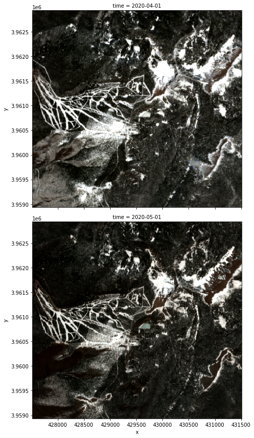
We’ll search for two months of Sentinel-2 data overlapping our area of interest—in this case, the Santa Fe ski area in New Mexico, USA (Google maps).
We use stackstac to create an xarray of all the data. From there, it’s easy to filter out cloudy scenes from the array based on their metadata, then create a median composite for each month.
[1]:
import stackstac
[2]:
lon, lat = -105.78, 35.79
We use pystac-client to find the relevant STAC (Spatio-Temporal Asset Catalog) items. These basically provide metadata about the relevant scenes, and links to their data.
We’ll use element84’s search endpoint to look for items from the sentinel-s2-l2a-cogs collection on AWS.
[3]:
import pystac_client
URL = "https://earth-search.aws.element84.com/v0"
catalog = pystac_client.Client.open(URL)
[4]:
%%time
items = catalog.search(
    intersects=dict(type="Point", coordinates=[lon, lat]),
    collections=["sentinel-s2-l2a-cogs"],
    datetime="2020-04-01/2020-05-01"
).get_all_items()
len(items)
CPU times: user 14.5 ms, sys: 3.2 ms, total: 17.7 ms
Wall time: 901 ms
[4]:
13
Use stackstac to turn those STAC items into a lazy xarray. Using all the defaults, our data will be in its native coordinate reference system, at the finest resolution of all the assets.
[5]:
%time stack = stackstac.stack(items)
CPU times: user 13.8 ms, sys: 1.88 ms, total: 15.7 ms
Wall time: 14.4 ms
[6]:
stack
[6]:
<xarray.DataArray 'stackstac-1949ba786c34763f8fa47e3f2f1d371a' (time: 13, band: 17, y: 10980, x: 10980)>
dask.array<fetch_raster_window, shape=(13, 17, 10980, 10980), dtype=float64, chunksize=(1, 1, 1024, 1024), chunktype=numpy.ndarray>
Coordinates: (12/24)
  * time                        (time) datetime64[ns] 2020-04-01T18:04:04 ......
    id                          (time) <U24 'S2B_13SDV_20200401_0_L2A' ... 'S...
  * band                        (band) <U8 'overview' 'visual' ... 'WVP' 'SCL'
  * x                           (x) float64 4e+05 4e+05 ... 5.097e+05 5.098e+05
  * y                           (y) float64 4e+06 4e+06 ... 3.89e+06 3.89e+06
    view:off_nadir              int64 0
    ...                          ...
    sentinel:data_coverage      (time) float64 33.85 100.0 33.9 ... 100.0 34.29
    proj:epsg                   int64 32613
    gsd                         int64 10
    sentinel:sequence           <U1 '0'
    title                       (band) object None ... 'Scene Classification ...
    epsg                        int64 32613
Attributes:
    spec:        RasterSpec(epsg=32613, bounds=(399960.0, 3890220.0, 509760.0...
    crs:         epsg:32613
    transform:   | 10.00, 0.00, 399960.00|\n| 0.00,-10.00, 4000020.00|\n| 0.0...
resolution: 10.0- time: 13
- band: 17
- y: 10980
- x: 10980
- dask.array<chunksize=(1, 1, 1024, 1024), meta=np.ndarray>
Array Chunk Bytes 198.51 GiB 8.00 MiB Shape (13, 17, 10980, 10980) (1, 1, 1024, 1024) Count 27304 Tasks 26741 Chunks Type float64 numpy.ndarray - time(time)datetime64[ns]2020-04-01T18:04:04 ... 2020-05-...
array(['2020-04-01T18:04:04.000000000', '2020-04-03T17:54:07.000000000', '2020-04-06T18:04:04.000000000', '2020-04-08T17:54:08.000000000', '2020-04-11T18:04:03.000000000', '2020-04-13T17:54:10.000000000', '2020-04-16T18:04:06.000000000', '2020-04-18T17:54:06.000000000', '2020-04-21T18:04:01.000000000', '2020-04-23T17:54:12.000000000', '2020-04-26T18:04:09.000000000', '2020-04-28T17:54:06.000000000', '2020-05-01T18:04:03.000000000'], dtype='datetime64[ns]') - id(time)<U24'S2B_13SDV_20200401_0_L2A' ... '...
array(['S2B_13SDV_20200401_0_L2A', 'S2A_13SDV_20200403_0_L2A', 'S2A_13SDV_20200406_0_L2A', 'S2B_13SDV_20200408_0_L2A', 'S2B_13SDV_20200411_0_L2A', 'S2A_13SDV_20200413_0_L2A', 'S2A_13SDV_20200416_0_L2A', 'S2B_13SDV_20200418_0_L2A', 'S2B_13SDV_20200421_0_L2A', 'S2A_13SDV_20200423_0_L2A', 'S2A_13SDV_20200426_0_L2A', 'S2B_13SDV_20200428_0_L2A', 'S2B_13SDV_20200501_0_L2A'], dtype='<U24') - band(band)<U8'overview' 'visual' ... 'WVP' 'SCL'
array(['overview', 'visual', 'B01', 'B02', 'B03', 'B04', 'B05', 'B06', 'B07', 'B08', 'B8A', 'B09', 'B11', 'B12', 'AOT', 'WVP', 'SCL'], dtype='<U8') - x(x)float644e+05 4e+05 ... 5.097e+05 5.098e+05
array([399960., 399970., 399980., ..., 509730., 509740., 509750.])
- y(y)float644e+06 4e+06 ... 3.89e+06 3.89e+06
array([4000020., 4000010., 4000000., ..., 3890250., 3890240., 3890230.])
- view:off_nadir()int640
array(0)
- instruments()<U3'msi'
array('msi', dtype='<U3') - sentinel:latitude_band()<U1'S'
array('S', dtype='<U1') - sentinel:product_id(time)<U60'S2B_MSIL2A_20200401T174909_N021...
array(['S2B_MSIL2A_20200401T174909_N0214_R141_T13SDV_20200401T220155', 'S2A_MSIL2A_20200403T173901_N0214_R098_T13SDV_20200403T220105', 'S2A_MSIL2A_20200406T174901_N0214_R141_T13SDV_20200406T221027', 'S2B_MSIL2A_20200408T173859_N0214_R098_T13SDV_20200408T215856', 'S2B_MSIL2A_20200411T174909_N0214_R141_T13SDV_20200411T220443', 'S2A_MSIL2A_20200413T173901_N0214_R098_T13SDV_20200413T235616', 'S2A_MSIL2A_20200416T174911_N0214_R141_T13SDV_20200416T221101', 'S2B_MSIL2A_20200418T173859_N0214_R098_T13SDV_20200418T214953', 'S2B_MSIL2A_20200421T174859_N0214_R141_T13SDV_20200421T214716', 'S2A_MSIL2A_20200423T173911_N0214_R098_T13SDV_20200423T234141', 'S2A_MSIL2A_20200426T174911_N0214_R141_T13SDV_20200426T221124', 'S2B_MSIL2A_20200428T173859_N0214_R098_T13SDV_20200428T214309', 'S2B_MSIL2A_20200501T174909_N0214_R141_T13SDV_20200501T220131'], dtype='<U60') - constellation()<U10'sentinel-2'
array('sentinel-2', dtype='<U10') - data_coverage(time)object33.85 100 33.9 ... 32.84 100 34.29
array([33.85, 100, 33.9, 100, 33.87, 100, 33.37, 100, 34.09, None, 32.84, 100, 34.29], dtype=object) - updated(time)<U24'2020-09-05T06:23:47.836Z' ... '...
array(['2020-09-05T06:23:47.836Z', '2020-09-23T15:43:10.502Z', '2020-09-05T11:18:48.722Z', '2020-08-31T15:23:56.855Z', '2020-09-23T16:16:43.693Z', '2020-09-24T06:31:45.567Z', '2020-09-24T05:31:29.634Z', '2020-09-19T07:13:25.290Z', '2020-09-05T11:20:20.745Z', '2020-08-23T09:50:31.532Z', '2020-09-05T13:56:08.881Z', '2020-08-31T13:13:14.956Z', '2020-09-24T07:38:40.841Z'], dtype='<U24') - sentinel:utm_zone()int6413
array(13)
- platform(time)<U11'sentinel-2b' ... 'sentinel-2b'
array(['sentinel-2b', 'sentinel-2a', 'sentinel-2a', 'sentinel-2b', 'sentinel-2b', 'sentinel-2a', 'sentinel-2a', 'sentinel-2b', 'sentinel-2b', 'sentinel-2a', 'sentinel-2a', 'sentinel-2b', 'sentinel-2b'], dtype='<U11') - sentinel:grid_square()<U2'DV'
array('DV', dtype='<U2') - eo:cloud_cover(time)float6429.24 1.16 27.26 ... 87.33 5.41
array([ 29.24, 1.16, 27.26, 1.15, 9.37, 100. , 4.53, 35. , 14.97, 31.78, 99.42, 87.33, 5.41]) - created(time)<U24'2020-09-05T06:23:47.836Z' ... '...
array(['2020-09-05T06:23:47.836Z', '2020-09-23T15:43:10.502Z', '2020-09-05T11:18:48.722Z', '2020-08-31T15:23:56.855Z', '2020-09-23T16:16:43.693Z', '2020-09-24T06:31:45.567Z', '2020-09-24T05:31:29.634Z', '2020-09-19T07:13:25.290Z', '2020-09-05T11:20:20.745Z', '2020-08-23T09:50:31.532Z', '2020-09-05T13:56:08.881Z', '2020-08-31T13:13:14.956Z', '2020-09-24T07:38:40.841Z'], dtype='<U24') - sentinel:valid_cloud_cover()boolTrue
array(True)
- sentinel:data_coverage(time)float6433.85 100.0 33.9 ... 100.0 34.29
array([ 33.85, 100. , 33.9 , 100. , 33.87, 100. , 33.37, 100. , 34.09, 100. , 32.84, 100. , 34.29]) - proj:epsg()int6432613
array(32613)
- gsd()int6410
array(10)
- sentinel:sequence()<U1'0'
array('0', dtype='<U1') - title(band)objectNone ... 'Scene Classification M...
array([None, 'True color image', 'Band 1 (coastal)', 'Band 2 (blue)', 'Band 3 (green)', 'Band 4 (red)', 'Band 5', 'Band 6', 'Band 7', 'Band 8 (nir)', 'Band 8A', 'Band 9', 'Band 11 (swir16)', 'Band 12 (swir22)', 'Aerosol Optical Thickness (AOT)', 'Water Vapour (WVP)', 'Scene Classification Map (SCL)'], dtype=object) - epsg()int6432613
array(32613)
- spec :
- RasterSpec(epsg=32613, bounds=(399960.0, 3890220.0, 509760.0, 4000020.0), resolutions_xy=(10.0, 10.0))
- crs :
- epsg:32613
- transform :
- | 10.00, 0.00, 399960.00| | 0.00,-10.00, 4000020.00| | 0.00, 0.00, 1.00|
- resolution :
- 10.0
Well, that’s really all there is to it. Now you have an xarray DataArray, and you can do whatever you like to it!
Here, we’ll filter out scenes with >20% cloud coverage (according to the eo:cloud_cover field set by the data provider). Then, pick the bands corresponding to red, green, and blue, and use xarray’s resample to create 1-month median composites.
[7]:
lowcloud = stack[stack["eo:cloud_cover"] < 20]
rgb = lowcloud.sel(band=["B04", "B03", "B02"])
monthly = rgb.resample(time="MS").median("time", keep_attrs=True)
[8]:
monthly
[8]:
<xarray.DataArray 'stackstac-1949ba786c34763f8fa47e3f2f1d371a' (time: 2, band: 3, y: 10980, x: 10980)>
dask.array<stack, shape=(2, 3, 10980, 10980), dtype=float64, chunksize=(1, 1, 1024, 1024), chunktype=numpy.ndarray>
Coordinates: (12/16)
  * time                        (time) datetime64[ns] 2020-04-01 2020-05-01
  * band                        (band) <U8 'B04' 'B03' 'B02'
  * x                           (x) float64 4e+05 4e+05 ... 5.097e+05 5.098e+05
  * y                           (y) float64 4e+06 4e+06 ... 3.89e+06 3.89e+06
    view:off_nadir              int64 0
    instruments                 <U3 'msi'
    ...                          ...
    sentinel:valid_cloud_cover  bool True
    proj:epsg                   int64 32613
    gsd                         int64 10
    sentinel:sequence           <U1 '0'
    title                       (band) object 'Band 4 (red)' ... 'Band 2 (blue)'
    epsg                        int64 32613
Attributes:
    spec:        RasterSpec(epsg=32613, bounds=(399960.0, 3890220.0, 509760.0...
    crs:         epsg:32613
    transform:   | 10.00, 0.00, 399960.00|\n| 0.00,-10.00, 4000020.00|\n| 0.0...
resolution: 10.0- time: 2
- band: 3
- y: 10980
- x: 10980
- dask.array<chunksize=(1, 1, 1024, 1024), meta=np.ndarray>
Array Chunk Bytes 5.39 GiB 8.00 MiB Shape (2, 3, 10980, 10980) (1, 1, 1024, 1024) Count 45817 Tasks 726 Chunks Type float64 numpy.ndarray - time(time)datetime64[ns]2020-04-01 2020-05-01
array(['2020-04-01T00:00:00.000000000', '2020-05-01T00:00:00.000000000'], dtype='datetime64[ns]') - band(band)<U8'B04' 'B03' 'B02'
array(['B04', 'B03', 'B02'], dtype='<U8')
- x(x)float644e+05 4e+05 ... 5.097e+05 5.098e+05
array([399960., 399970., 399980., ..., 509730., 509740., 509750.])
- y(y)float644e+06 4e+06 ... 3.89e+06 3.89e+06
array([4000020., 4000010., 4000000., ..., 3890250., 3890240., 3890230.])
- view:off_nadir()int640
array(0)
- instruments()<U3'msi'
array('msi', dtype='<U3') - sentinel:latitude_band()<U1'S'
array('S', dtype='<U1') - constellation()<U10'sentinel-2'
array('sentinel-2', dtype='<U10') - sentinel:utm_zone()int6413
array(13)
- sentinel:grid_square()<U2'DV'
array('DV', dtype='<U2') - sentinel:valid_cloud_cover()boolTrue
array(True)
- proj:epsg()int6432613
array(32613)
- gsd()int6410
array(10)
- sentinel:sequence()<U1'0'
array('0', dtype='<U1') - title(band)object'Band 4 (red)' ... 'Band 2 (blue)'
array(['Band 4 (red)', 'Band 3 (green)', 'Band 2 (blue)'], dtype=object)
- epsg()int6432613
array(32613)
- spec :
- RasterSpec(epsg=32613, bounds=(399960.0, 3890220.0, 509760.0, 4000020.0), resolutions_xy=(10.0, 10.0))
- crs :
- epsg:32613
- transform :
- | 10.00, 0.00, 399960.00| | 0.00,-10.00, 4000020.00| | 0.00, 0.00, 1.00|
- resolution :
- 10.0
So we don’t pull all ~200 GB of data down to our local machine, let’s slice out a little region around our area of interest.
We convert our lat-lon point to the data’s UTM coordinate reference system, then use that to slice the x and y dimensions, which are indexed by their UTM coordinates.
[9]:
import pyproj
x_utm, y_utm = pyproj.Proj(monthly.crs)(lon, lat)
buffer = 2000  # meters
[10]:
aoi = monthly.loc[..., y_utm+buffer:y_utm-buffer, x_utm-buffer:x_utm+buffer]
aoi
[10]:
<xarray.DataArray 'stackstac-1949ba786c34763f8fa47e3f2f1d371a' (time: 2, band: 3, y: 400, x: 400)>
dask.array<getitem, shape=(2, 3, 400, 400), dtype=float64, chunksize=(1, 1, 387, 316), chunktype=numpy.ndarray>
Coordinates: (12/16)
  * time                        (time) datetime64[ns] 2020-04-01 2020-05-01
  * band                        (band) <U8 'B04' 'B03' 'B02'
  * x                           (x) float64 4.275e+05 4.275e+05 ... 4.315e+05
  * y                           (y) float64 3.963e+06 3.963e+06 ... 3.959e+06
    view:off_nadir              int64 0
    instruments                 <U3 'msi'
    ...                          ...
    sentinel:valid_cloud_cover  bool True
    proj:epsg                   int64 32613
    gsd                         int64 10
    sentinel:sequence           <U1 '0'
    title                       (band) object 'Band 4 (red)' ... 'Band 2 (blue)'
    epsg                        int64 32613
Attributes:
    spec:        RasterSpec(epsg=32613, bounds=(399960.0, 3890220.0, 509760.0...
    crs:         epsg:32613
    transform:   | 10.00, 0.00, 399960.00|\n| 0.00,-10.00, 4000020.00|\n| 0.0...
resolution: 10.0- time: 2
- band: 3
- y: 400
- x: 400
- dask.array<chunksize=(1, 1, 387, 316), meta=np.ndarray>
Array Chunk Bytes 7.32 MiB 0.93 MiB Shape (2, 3, 400, 400) (1, 1, 387, 316) Count 45841 Tasks 24 Chunks Type float64 numpy.ndarray - time(time)datetime64[ns]2020-04-01 2020-05-01
array(['2020-04-01T00:00:00.000000000', '2020-05-01T00:00:00.000000000'], dtype='datetime64[ns]') - band(band)<U8'B04' 'B03' 'B02'
array(['B04', 'B03', 'B02'], dtype='<U8')
- x(x)float644.275e+05 4.275e+05 ... 4.315e+05
array([427520., 427530., 427540., ..., 431490., 431500., 431510.])
- y(y)float643.963e+06 3.963e+06 ... 3.959e+06
array([3962930., 3962920., 3962910., ..., 3958960., 3958950., 3958940.])
- view:off_nadir()int640
array(0)
- instruments()<U3'msi'
array('msi', dtype='<U3') - sentinel:latitude_band()<U1'S'
array('S', dtype='<U1') - constellation()<U10'sentinel-2'
array('sentinel-2', dtype='<U10') - sentinel:utm_zone()int6413
array(13)
- sentinel:grid_square()<U2'DV'
array('DV', dtype='<U2') - sentinel:valid_cloud_cover()boolTrue
array(True)
- proj:epsg()int6432613
array(32613)
- gsd()int6410
array(10)
- sentinel:sequence()<U1'0'
array('0', dtype='<U1') - title(band)object'Band 4 (red)' ... 'Band 2 (blue)'
array(['Band 4 (red)', 'Band 3 (green)', 'Band 2 (blue)'], dtype=object)
- epsg()int6432613
array(32613)
- spec :
- RasterSpec(epsg=32613, bounds=(399960.0, 3890220.0, 509760.0, 4000020.0), resolutions_xy=(10.0, 10.0))
- crs :
- epsg:32613
- transform :
- | 10.00, 0.00, 399960.00| | 0.00,-10.00, 4000020.00| | 0.00, 0.00, 1.00|
- resolution :
- 10.0
[11]:
import dask.diagnostics
with dask.diagnostics.ProgressBar():
    data = aoi.compute()
[########################################] | 100% Completed | 12.1s
[12]:
data.plot.imshow(row="time", rgb="band", robust=True, size=6);