Note
You can view & download the original notebook on Github.
Or, click here to run these notebooks on Coiled with access to Dask clusters.
Stacking 6 years of imagery into a GIF
We’ll load all the Landsat-8 (Collection 2, Level 2) data that’s available from Microsoft’s Planetary Computer over a small region on the coast of Cape Cod, Massachusetts, USA.
Using nothing but standard xarray syntax, we’ll mask cloudy pixels with the Landsat QA band and reduce the data down to biannual median composites.
Animated as a GIF, we can watch the coastline move over the years due to longshore drift.
Planetary Computer is Microsoft’s open Earth data initiative. It’s particularly nice to use, since they also maintain a STAC API for searching all the data, as well as a browseable data catalog. It’s free for anyone to use, though you have to sign your requests with the planetary_computer package to
prevent abuse. If you sign up, you’ll get faster reads.
[1]:
import coiled
import distributed
import dask
import pystac_client
import planetary_computer as pc
import ipyleaflet
import IPython.display as dsp
import geogif
import stackstac
Using a cluster will make this much faster. Particularly if you’re not in Europe, which is where this data is stored.
You can sign up for a Coiled account and run clusters for free at https://cloud.coiled.io/ — no credit card or username required, just sign in with your GitHub or Google account.
[2]:
cluster = coiled.Cluster(
    name="stackstac-eu",
    software="gjoseph92/stackstac",
    backend_options={"region": "eu-central-1"},
    # ^ Coiled doesn't yet support Azure's West Europe region, so instead we'll run on a nearby AWS data center in Frankfurt
    n_workers=20,
)
client = distributed.Client(cluster)
client
Using existing cluster: 'stackstac'
[2]:
Client
|
Cluster
|
Interactively pick the area of interest from a map. Just move the map around and re-run all cells to generate the timeseries somewhere else!
[3]:
m = ipyleaflet.Map(scroll_wheel_zoom=True)
m.center = 41.64933994767867, -69.94438630063088
m.zoom = 12
m.layout.height = "800px"
m
[4]:
bbox = (m.west, m.south, m.east, m.north)
Search for STAC items
Use pystac-client to connect to Microsoft’s STAC API endpoint and search for Landsat-8 scenes.
[5]:
catalog = pystac_client.Client.open('https://planetarycomputer.microsoft.com/api/stac/v1')

search = catalog.search(
    collections=['landsat-8-c2-l2'],
    bbox=bbox,
)
search.matched()
[5]:
357
[6]:
%%time
items = search.items_as_collection()
CPU times: user 719 ms, sys: 45.7 ms, total: 764 ms
Wall time: 15.2 s
Sign all the STAC items with a token from Planetary Computer. Without this, loading the data will fail.
[7]:
items = pystac_client.ItemCollection([pc.sign_assets(item) for item in items.features])
These are the footprints of all the items we’ll use:
[ ]:
dsp.GeoJSON(items.to_dict())
Create an xarray with stacksatc
Set bounds_latlon=bbox to automatically clip to our area of interest (instead of using the full footprints of the scenes).
[9]:
%%time
stack = stackstac.stack(items, bounds_latlon=bbox)
stack
CPU times: user 362 ms, sys: 11.4 ms, total: 374 ms
Wall time: 372 ms
[9]:
<xarray.DataArray 'stackstac-9678efaf932b81b94aa1dceb9a89fb92' (time: 357, band: 19, y: 774, x: 1261)>
dask.array<fetch_raster_window, shape=(357, 19, 774, 1261), dtype=float64, chunksize=(1, 1, 774, 1024), chunktype=numpy.ndarray>
Coordinates: (12/26)
  * time                         (time) datetime64[ns] 2013-03-22T15:19:00.54...
    id                           (time) <U40 'LC08_L2SP_011031_20130322_20200...
  * band                         (band) <U9 'QA_PIXEL' 'QA_RADSAT' ... 'ST_QA'
  * x                            (x) float64 4.024e+05 4.025e+05 ... 4.402e+05
  * y                            (y) float64 4.623e+06 4.623e+06 ... 4.6e+06
    landsat:collection_category  (time) object None None None ... 'T2' 'T1' 'T1'
    ...                           ...
    view:sun_azimuth             (time) float64 149.6 148.3 ... 153.9 149.3
    gsd                          (band) object None None None ... 30.0 30.0 30.0
    title                        (band) <U46 'Pixel Quality Assessment Band' ...
    common_name                  (band) object None None 'coastal' ... None None
    center_wavelength            (band) object None None 0.44 ... None None None
    full_width_half_max          (band) object None None 0.02 ... None None None
Attributes:
    spec:           RasterSpec(epsg=32619, bounds=(402426.3431542461, 4599672...
    crs:            epsg:32619
    transform:      | 30.00, 0.00, 402426.34|\n| 0.00,-30.00, 4622889.48|\n| ...
resolution_xy: (29.996000533262233, 29.995973694806068)- time: 357
- band: 19
- y: 774
- x: 1261
- dask.array<chunksize=(1, 1, 774, 1024), meta=np.ndarray>
Array Chunk Bytes 49.33 GiB 6.05 MiB Shape (357, 19, 774, 1261) (1, 1, 774, 1024) Count 27134 Tasks 13566 Chunks Type float64 numpy.ndarray - time(time)datetime64[ns]2013-03-22T15:19:00.545659 ... 2...
array(['2013-03-22T15:19:00.545659000', '2013-04-04T15:27:44.408822000', '2013-04-09T15:27:54.193621000', ..., '2021-01-16T15:27:16.497121000', '2021-02-10T15:21:01.910838000', '2021-03-21T15:26:55.644963000'], dtype='datetime64[ns]') - id(time)<U40'LC08_L2SP_011031_20130322_20200...
array(['LC08_L2SP_011031_20130322_20200912_02_T1', 'LC08_L2SP_012031_20130404_20200913_02_T1', 'LC08_L2SP_012031_20130409_20200913_02_T1', 'LC08_L2SP_012031_20130416_20200913_02_T1', 'LC08_L2SP_012031_20130502_20200913_02_T1', 'LC08_L2SP_011031_20130511_20200912_02_T1', 'LC08_L2SP_012031_20130518_20200913_02_T1', 'LC08_L2SP_011031_20130527_20200913_02_T1', 'LC08_L2SP_012031_20130603_20200912_02_T2', 'LC08_L2SP_012031_20130619_20200912_02_T1', 'LC08_L2SP_011031_20130628_20200912_02_T2', 'LC08_L2SP_012031_20130705_20200912_02_T1', 'LC08_L2SP_011031_20130714_20200912_02_T1', 'LC08_L2SP_012031_20130721_20200912_02_T1', 'LC08_L2SP_011031_20130730_20200912_02_T1', 'LC08_L2SP_012031_20130806_20200912_02_T1', 'LC08_L2SP_011031_20130815_20200913_02_T1', 'LC08_L2SP_012031_20130822_20200912_02_T1', 'LC08_L2SP_011031_20130831_20200912_02_T1', 'LC08_L2SP_012031_20130907_20200913_02_T1', ... 'LC08_L2SP_012031_20200825_20200905_02_T1', 'LC08_L2SP_011031_20200903_20200918_02_T2', 'LC08_L2SP_012031_20200910_20200919_02_T2', 'LC08_L2SP_011031_20200919_20201006_02_T1', 'LC08_L2SP_012031_20200926_20201006_02_T1', 'LC08_L2SP_011031_20201005_20201016_02_T2', 'LC08_L2SP_012031_20201012_20201105_02_T2', 'LC08_L2SP_011031_20201021_20201106_02_T2', 'LC08_L2SP_012031_20201028_20201106_02_T2', 'LC08_L2SP_011031_20201122_20201210_02_T2', 'LC08_L2SP_012031_20201129_20201211_02_T1', 'LC08_L2SP_011031_20201208_20210313_02_T1', 'LC08_L2SP_011031_20201208_20201218_02_T1', 'LC08_L2SP_012031_20201215_20210314_02_T1', 'LC08_L2SP_012031_20201215_20201219_02_T1', 'LC08_L2SP_011031_20201224_20210310_02_T1', 'LC08_L2SP_012031_20201231_20210308_02_T2', 'LC08_L2SP_012031_20210116_20210306_02_T2', 'LC08_L2SP_011031_20210210_20210302_02_T1', 'LC08_L2SP_012031_20210321_20210401_02_T1'], dtype='<U40') - band(band)<U9'QA_PIXEL' 'QA_RADSAT' ... 'ST_QA'
array(['QA_PIXEL', 'QA_RADSAT', 'SR_B1', 'SR_B2', 'SR_B3', 'SR_B4', 'SR_B5', 'SR_B6', 'SR_B7', 'SR_B8', 'ST_B10', 'ST_ATRAN', 'ST_CDIST', 'ST_DRAD', 'ST_URAD', 'ST_TRAD', 'ST_EMIS', 'ST_EMSD', 'ST_QA'], dtype='<U9') - x(x)float644.024e+05 4.025e+05 ... 4.402e+05
array([402441.341155, 402471.337155, 402501.333156, ..., 440176.309825, 440206.305826, 440236.301826]) - y(y)float644.623e+06 4.623e+06 ... 4.6e+06
array([4622904.475909, 4622874.479936, 4622844.483962, ..., 4599777.580191, 4599747.584217, 4599717.588243]) - landsat:collection_category(time)objectNone None None ... 'T2' 'T1' 'T1'
array([None, None, None, None, None, None, None, 'T1', 'T2', 'T1', 'T2', 'T1', 'T1', 'T1', 'T1', 'T1', 'T1', 'T1', 'T1', 'T1', 'T2', 'T1', 'T1', 'T1', 'T2', 'T1', 'T1', 'T2', 'T2', 'T1', 'T1', 'T1', 'T2', 'T1', 'T2', 'T1', 'T1', 'T1', 'T1', 'T2', 'T1', 'T1', 'T1', 'T1', 'T1', 'T1', 'T1', 'T1', 'T1', 'T1', 'T1', 'T1', 'T1', 'T1', 'T1', 'T1', 'T1', 'T1', 'T2', 'T1', 'T1', 'T1', 'T1', 'T1', 'T1', 'T1', 'T1', 'T1', 'T1', 'T1', 'T2', 'T1', 'T1', 'T1', 'T2', 'T1', 'T2', 'T1', 'T2', 'T1', 'T1', 'T1', 'T2', 'T2', 'T2', 'T2', 'T2', 'T2', 'T1', 'T1', 'T2', 'T2', 'T1', 'T1', 'T1', 'T1', 'T1', 'T2', 'T2', 'T1', 'T1', 'T2', 'T1', 'T1', 'T1', 'T1', 'T1', 'T1', 'T1', 'T1', 'T2', 'T1', 'T1', 'T1', 'T1', 'T2', 'T1', 'T1', 'T1', 'T1', 'T2', 'T1', 'T2', 'T2', 'T1', 'T1', 'T1', 'T1', 'T2', 'T1', 'T1', 'T1', 'T1', 'T2', 'T1', 'T2', 'T1', 'T1', 'T1', 'T2', 'T1', 'T1', 'T1', 'T1', 'T1', 'T1', 'T1', 'T1', 'T1', 'T1', 'T2', 'T1', 'T1', 'T1', 'T1', 'T2', 'T1', 'T1', 'T2', 'T1', 'T1', 'T1', 'T1', 'T1', 'T1', 'T1', 'T1', 'T1', 'T1', 'T2', 'T1', 'T1', 'T2', 'T1', 'T1', 'T2', 'T1', 'T1', 'T2', 'T2', 'T1', 'T2', 'T1', 'T2', 'T2', 'T2', 'T2', 'T2', 'T2', 'T1', 'T1', 'T1', 'T1', 'T1', 'T1', 'T2', 'T1', 'T1', 'T1', 'T1', 'T1', 'T1', 'T2', 'T1', 'T1', 'T1', 'T1', 'T2', 'T2', 'T2', 'T1', 'T1', 'T1', 'T1', 'T2', 'T1', 'T1', 'T2', 'T1', 'T2', 'T1', 'T1', 'T2', 'T2', 'T2', 'T2', 'T1', 'T1', 'T1', 'T1', 'T2', 'T1', 'T1', 'T1', 'T2', 'T1', 'T1', 'T1', 'T1', 'T1', 'T1', 'T1', 'T2', 'T2', 'T1', 'T1', 'T1', 'T1', 'T1', 'T1', 'T2', 'T1', 'T2', 'T1', 'T1', 'T1', 'T1', 'T1', 'T1', 'T1', 'T1', 'T1', 'T1', 'T2', 'T1', 'T1', 'T2', 'T2', 'T1', 'T1', 'T1', 'T1', 'T1', 'T1', 'T1', 'T2', 'T1', 'T2', 'T1', 'T2', 'T1', 'T2', 'T2', 'T1', 'T1', 'T1', 'T1', 'T1', 'T1', 'T1', 'T2', 'T1', 'T1', 'T1', 'T1', 'T2', 'T2', 'T1', 'T1', 'T1', 'T1', 'T2', 'T2', 'T2', 'T1', 'T1', 'T1', 'T1', 'T1', 'T1', 'T1', 'T1', 'T1', 'T1', 'T1', 'T1', 'T1', 'T1', 'T1', 'T2', 'T1', 'T1', 'T2', 'T1', 'T1', 'T1', 'T1', 'T1', 'T1', 'T1', 'T1', 'T1', 'T2', 'T1', 'T1', 'T1', 'T1', 'T1', 'T2', 'T2', 'T1', 'T1', 'T2', 'T2', 'T2', 'T2', 'T2', 'T1', 'T1', 'T1', 'T1', 'T1', 'T1', 'T2', 'T2', 'T1', 'T1'], dtype=object) - description(band)<U91'Collection 2 Level-1 Pixel Qual...
array(['Collection 2 Level-1 Pixel Quality Assessment Band', 'Collection 2 Level-1 Radiometric Saturation Quality Assessment Band', 'Collection 2 Level-2 Coastal/Aerosol Band (B1) Surface Reflectance', 'Collection 2 Level-2 Blue Band (B2) Surface Reflectance', 'Collection 2 Level-2 Green Band (B3) Surface Reflectance', 'Collection 2 Level-2 Red Band (B4) Surface Reflectance', 'Collection 2 Level-2 Near Infrared Band 0.8 (B5) Surface Reflectance', 'Collection 2 Level-2 Short-wave Infrared Band 1.6 (B6) Surface Reflectance', 'Collection 2 Level-2 Short-wave Infrared Band 2.2 (B7) Surface Reflectance', 'Collection 2 Level-2 Aerosol Quality Analysis Band (ANG) Surface Reflectance', 'Landsat Collection 2 Level-2 Surface Temperature Band (B10) Surface Temperature Product', 'Landsat Collection 2 Level-2 Atmospheric Transmittance Band Surface Temperature Product', 'Landsat Collection 2 Level-2 Cloud Distance Band Surface Temperature Product', 'Landsat Collection 2 Level-2 Downwelled Radiance Band Surface Temperature Product', 'Landsat Collection 2 Level-2 Upwelled Radiance Band Surface Temperature Product', 'Landsat Collection 2 Level-2 Thermal Radiance Band Surface Temperature Product', 'Landsat Collection 2 Level-2 Emissivity Band Surface Temperature Product', 'Landsat Collection 2 Level-2 Emissivity Standard Deviation Band Surface Temperature Product', 'Landsat Collection 2 Level-2 Surface Temperature Band Surface Temperature Product'], dtype='<U91') - landsat8:scene_id(time)<U21'LC80110312013081LGN02' ... 'LC8...
array(['LC80110312013081LGN02', 'LC80120312013094LGN02', 'LC80120312013099LGN02', 'LC80120312013106LGN03', 'LC80120312013122LGN02', 'LC80110312013131LGN02', 'LC80120312013138LGN02', 'LC80110312013147LGN01', 'LC80120312013154LGN01', 'LC80120312013170LGN01', 'LC80110312013179LGN01', 'LC80120312013186LGN01', 'LC80110312013195LGN01', 'LC80120312013202LGN01', 'LC80110312013211LGN01', 'LC80120312013218LGN01', 'LC80110312013227LGN01', 'LC80120312013234LGN01', 'LC80110312013243LGN01', 'LC80120312013250LGN01', 'LC80110312013259LGN01', 'LC80120312013266LGN01', 'LC80110312013275LGN01', 'LC80110312013291LGN01', 'LC80110312013307LGN01', 'LC80120312013314LGN01', 'LC80110312013323LGN01', 'LC80120312013330LGN01', 'LC80110312013339LGN04', 'LC80120312013346LGN01', 'LC80110312013355LGN02', 'LC80120312013362LGN01', 'LC80110312014006LGN01', 'LC80120312014013LGN01', 'LC80110312014022LGN01', 'LC80120312014029LGN01', 'LC80110312014038LGN01', 'LC80120312014045LGN01', 'LC80110312014054LGN01', 'LC80120312014061LGN03', ... 'LC80110312020087LGN00', 'LC80120312020094LGN00', 'LC80110312020103LGN00', 'LC80120312020110LGN00', 'LC80110312020119LGN00', 'LC80120312020126LGN00', 'LC80110312020135LGN00', 'LC80120312020142LGN00', 'LC80110312020151LGN00', 'LC80120312020158LGN00', 'LC80110312020167LGN00', 'LC80120312020174LGN00', 'LC80110312020183LGN00', 'LC80120312020190LGN00', 'LC80110312020199LGN00', 'LC80120312020206LGN00', 'LC80110312020215LGN00', 'LC80120312020222LGN00', 'LC80110312020231LGN00', 'LC80120312020238LGN00', 'LC80110312020247LGN00', 'LC80120312020254LGN00', 'LC80110312020263LGN00', 'LC80120312020270LGN00', 'LC80110312020279LGN00', 'LC80120312020286LGN00', 'LC80110312020295LGN00', 'LC80120312020302LGN00', 'LC80110312020327LGN00', 'LC80120312020334LGN00', 'LC80110312020343LGN00', 'LC80110312020343LGN00', 'LC80120312020350LGN00', 'LC80120312020350LGN00', 'LC80110312020359LGN00', 'LC80120312020366LGN00', 'LC80120312021016LGN00', 'LC80110312021041LGN00', 'LC80120312021080LGN00'], dtype='<U21') - eo:cloud_cover(time)float6492.94 0.77 11.81 ... 48.61 0.18
array([9.294e+01, 7.700e-01, 1.181e+01, 1.176e+01, 8.000e-02, 9.830e+01, 6.145e+01, 3.610e+00, 3.849e+01, 1.485e+01, 9.701e+01, 4.060e+00, 6.344e+01, 8.257e+01, 3.419e+01, 3.300e-01, 1.700e-01, 7.695e+01, 3.617e+01, 9.500e-01, 3.669e+01, 1.500e-01, 1.180e+00, 1.490e+00, 1.000e+02, 5.575e+01, 7.640e+01, 1.000e+02, 9.996e+01, 8.820e+00, 9.412e+01, 8.389e+01, 1.000e+02, 2.059e+01, 1.000e+02, 5.240e+01, 2.650e+00, 7.982e+01, 7.669e+01, 9.993e+01, 9.902e+01, 7.130e+00, 3.000e-01, 1.470e+00, 7.100e-01, 8.950e+00, 7.563e+01, 6.817e+01, 5.917e+01, 1.160e+01, 1.895e+01, 3.335e+01, 2.505e+01, 2.029e+01, 8.351e+01, 8.238e+01, 8.675e+01, 8.787e+01, 1.000e+02, 1.640e+00, 1.060e+01, 4.000e-02, 4.884e+01, 7.218e+01, 2.226e+01, 2.037e+01, 3.300e+01, 6.100e-01, 9.848e+01, 4.360e+01, 1.000e+02, 1.197e+01, 3.529e+01, 2.480e+00, 9.579e+01, 1.663e+01, 1.000e+02, 3.445e+01, 1.000e+02, 3.486e+01, 5.810e+00, 9.600e+00, 1.000e+02, 1.000e+02, 1.000e+02, 1.000e+02, 9.997e+01, 1.000e+02, 8.473e+01, 1.334e+01, 9.197e+01, 9.197e+01, 3.011e+01, 3.286e+01, 3.286e+01, 5.800e-01, 5.800e-01, 9.996e+01, 9.996e+01, 9.759e+01, 7.780e+00, 1.000e+02, 4.380e+00, 3.274e+01, 8.686e+01, 6.320e+01, 2.147e+01, 8.024e+01, 6.680e+00, 2.000e-02, 1.620e+01, 9.358e+01, 5.647e+01, 2.360e+00, 1.340e+00, 9.999e+01, 1.780e+00, 1.000e-02, 8.670e+00, 4.440e+00, ... 4.400e-01, 7.727e+01, 3.756e+01, 9.530e+01, 7.331e+01, 5.740e+00, 7.920e+00, 2.120e+01, 3.022e+01, 1.370e+00, 8.983e+01, 2.777e+01, 5.282e+01, 5.223e+01, 4.996e+01, 2.512e+01, 4.123e+01, 7.132e+01, 1.298e+01, 1.638e+01, 3.410e+00, 2.889e+01, 1.280e+00, 1.000e+02, 1.846e+01, 4.467e+01, 1.000e+02, 8.806e+01, 6.074e+01, 6.000e-02, 2.426e+01, 7.706e+01, 3.270e+00, 6.860e+01, 3.000e-02, 1.000e+02, 8.406e+01, 9.999e+01, 9.481e+01, 9.624e+01, 1.829e+01, 9.999e+01, 1.000e+02, 9.796e+01, 4.523e+01, 5.436e+01, 7.694e+01, 1.207e+01, 8.059e+01, 5.325e+01, 9.530e+01, 3.371e+01, 2.893e+01, 1.698e+01, 1.924e+01, 6.010e+01, 9.887e+01, 1.900e+01, 1.113e+01, 3.400e-01, 4.317e+01, 9.993e+01, 1.000e+02, 5.526e+01, 9.535e+01, 9.548e+01, 7.173e+01, 2.764e+01, 7.966e+01, 9.807e+01, 5.900e-01, 6.020e+00, 8.430e+00, 2.700e+00, 6.000e-02, 4.819e+01, 2.080e+00, 1.220e+00, 4.293e+01, 1.000e+02, 2.141e+01, 2.570e+00, 9.932e+01, 2.490e+00, 3.100e-01, 3.300e-01, 7.558e+01, 7.017e+01, 5.567e+01, 6.878e+01, 7.090e+01, 5.123e+01, 9.915e+01, 8.513e+01, 2.198e+01, 1.577e+01, 9.420e+00, 4.708e+01, 8.784e+01, 1.000e+02, 6.930e+00, 3.368e+01, 9.557e+01, 5.380e+01, 8.696e+01, 1.000e+02, 9.426e+01, 1.700e-01, 9.934e+01, 9.934e+01, 2.300e+00, 2.240e+00, 1.757e+01, 1.000e+02, 7.411e+01, 4.861e+01, 1.800e-01]) - landsat:wrs_type()<U1'2'
array('2', dtype='<U1') - landsat:cloud_cover_land(time)float6490.98 1.51 15.5 ... 25.88 0.29
array([9.098e+01, 1.510e+00, 1.550e+01, 1.483e+01, 9.000e-02, 9.785e+01, 6.750e+01, 1.350e+00, 4.337e+01, 7.410e+00, 8.166e+01, 5.490e+00, 2.527e+01, 8.131e+01, 1.500e-01, 5.800e-01, 8.200e-01, 7.823e+01, 3.148e+01, 1.460e+00, 4.881e+01, 2.500e-01, 1.570e+00, 7.500e-01, 1.000e+02, 5.482e+01, 7.518e+01, 1.000e+02, 1.000e+02, 7.080e+00, 9.790e+01, 8.688e+01, 1.000e+02, 3.339e+01, 1.000e+02, 2.661e+01, 8.780e+00, 8.246e+01, 7.588e+01, 9.987e+01, 9.804e+01, 1.219e+01, 3.270e+00, 2.100e+00, 2.500e-01, 4.650e+00, 5.056e+01, 8.494e+01, 5.551e+01, 1.009e+01, 5.100e-01, 4.320e+01, 2.203e+01, 2.587e+01, 9.673e+01, 9.012e+01, 7.491e+01, 8.613e+01, 1.000e+02, 2.820e+00, 2.400e+01, 6.000e-02, 5.112e+01, 7.882e+01, 1.255e+01, 6.100e+00, 4.000e-02, 1.600e-01, 9.939e+01, 3.680e+01, 1.000e+02, 2.044e+01, 2.975e+01, 3.830e+00, 9.999e+01, 4.810e+00, 1.000e+02, 2.449e+01, 1.000e+02, 2.255e+01, 1.230e+01, 8.810e+00, 9.999e+01, 1.000e+02, 1.000e+02, 1.000e+02, 1.000e+02, 1.000e+02, 8.824e+01, 1.030e+00, 9.920e+01, 9.920e+01, 7.300e+00, 9.750e+00, 9.750e+00, 1.600e-01, 1.600e-01, 1.000e+02, 9.999e+01, 8.625e+01, 1.325e+01, 1.000e+02, 7.600e-01, 1.970e+00, 8.008e+01, 2.190e+01, 2.370e+01, 9.902e+01, 1.171e+01, 1.600e-01, 2.200e+00, 8.713e+01, 6.033e+01, 1.228e+01, 2.900e-01, 1.000e+02, 9.500e-01, 1.300e-01, 1.430e+00, 2.290e+00, ... 1.200e-01, 5.778e+01, 4.545e+01, 9.947e+01, 6.368e+01, 3.000e-01, 1.025e+01, 3.401e+01, 4.950e+01, 5.000e-01, 9.241e+01, 4.012e+01, 6.076e+01, 6.168e+01, 4.184e+01, 1.737e+01, 4.576e+01, 5.355e+01, 4.900e+00, 6.510e+00, 3.100e+00, 2.893e+01, 1.660e+00, 1.000e+02, 3.114e+01, 5.563e+01, 1.000e+02, 9.958e+01, 5.040e+01, 6.700e-01, 3.726e+01, 8.770e+01, 5.500e+00, 7.790e+01, 4.000e-02, 1.000e+02, 7.805e+01, 1.000e+02, 9.728e+01, 9.915e+01, 2.690e+01, 1.000e+02, 1.000e+02, 9.149e+01, 4.081e+01, 1.789e+01, 8.684e+01, 4.500e-01, 8.793e+01, 1.678e+01, 9.496e+01, 1.838e+01, 3.599e+01, 1.309e+01, 3.254e+01, 6.500e+01, 9.804e+01, 2.230e+00, 1.395e+01, 5.300e-01, 5.418e+01, 1.000e+02, 1.000e+02, 8.843e+01, 9.999e+01, 9.999e+01, 9.934e+01, 3.538e+01, 8.829e+01, 9.666e+01, 5.570e+00, 4.920e+00, 4.500e-01, 4.520e+00, 4.600e-01, 7.137e+01, 1.050e+00, 2.130e+00, 2.580e+01, 1.000e+02, 5.164e+01, 4.420e+00, 9.723e+01, 1.150e+00, 5.000e-01, 1.000e-01, 3.439e+01, 5.539e+01, 6.356e+01, 5.995e+01, 8.879e+01, 7.155e+01, 9.997e+01, 8.073e+01, 5.321e+01, 2.524e+01, 8.480e+00, 5.610e+01, 9.960e+01, 9.999e+01, 1.611e+01, 2.704e+01, 9.998e+01, 4.007e+01, 9.715e+01, 1.000e+02, 1.000e+02, 2.900e-01, 9.918e+01, 9.918e+01, 3.780e+00, 3.670e+00, 1.641e+01, 1.000e+02, 7.747e+01, 2.588e+01, 2.900e-01]) - platform()<U9'landsat-8'
array('landsat-8', dtype='<U9') - view:off_nadir()int640
array(0)
- landsat:wrs_row()<U3'031'
array('031', dtype='<U3') - landsat:collection_number()<U2'02'
array('02', dtype='<U2') - landsat:processing_level()<U4'L2SP'
array('L2SP', dtype='<U4') - landsat:wrs_path(time)<U3'011' '012' '012' ... '011' '012'
array(['011', '012', '012', '012', '012', '011', '012', '011', '012', '012', '011', '012', '011', '012', '011', '012', '011', '012', '011', '012', '011', '012', '011', '011', '011', '012', '011', '012', '011', '012', '011', '012', '011', '012', '011', '012', '011', '012', '011', '012', '011', '012', '011', '012', '011', '012', '011', '012', '011', '012', '011', '012', '011', '012', '011', '012', '011', '012', '011', '012', '011', '012', '011', '012', '011', '012', '011', '012', '011', '012', '011', '012', '011', '012', '011', '012', '011', '012', '011', '012', '011', '012', '012', '011', '012', '011', '012', '011', '012', '011', '011', '011', '012', '011', '011', '012', '012', '011', '012', '011', '012', '011', '012', '011', '012', '011', '012', '011', '012', '011', '012', '011', '012', '011', '012', '011', '012', '011', '012', '011', '012', '011', '012', '011', '012', '011', '012', '011', '012', '011', '012', '011', '012', '011', '012', '011', '012', '011', '012', '011', '012', '011', '012', '011', '012', '011', '012', '011', '012', '011', '012', '011', '012', '011', '012', '011', '012', '011', '012', '011', '012', '011', '012', '011', '012', '011', '012', '011', '012', '011', '012', '011', '012', '011', '012', '011', '012', '011', '012', '011', '012', '011', '012', '011', '012', '011', '012', '011', '012', '011', '012', '011', '012', '011', '012', '011', '012', '011', '012', '011', '012', '011', '012', '011', '012', '011', '012', '011', '012', '011', '012', '011', '012', '011', '012', '011', '012', '011', '012', '011', '012', '011', '012', '011', '012', '011', '012', '011', '012', '011', '012', '011', '012', '011', '012', '011', '012', '011', '012', '011', '012', '011', '012', '011', '012', '011', '012', '011', '012', '011', '012', '011', '012', '011', '012', '011', '012', '011', '012', '011', '012', '011', '012', '011', '012', '011', '012', '011', '012', '011', '012', '011', '012', '011', '012', '011', '012', '011', '012', '011', '012', '011', '012', '011', '012', '011', '012', '011', '012', '011', '012', '011', '012', '011', '012', '011', '012', '011', '012', '011', '012', '011', '012', '011', '012', '012', '011', '012', '011', '012', '011', '012', '011', '012', '011', '012', '011', '012', '011', '012', '011', '012', '011', '012', '011', '012', '011', '012', '011', '012', '011', '012', '011', '012', '011', '012', '011', '012', '011', '012', '011', '012', '011', '012', '011', '012', '011', '012', '011', '011', '012', '012', '011', '012', '012', '011', '012'], dtype='<U3') - proj:epsg()int6432619
array(32619)
- view:sun_elevation(time)float6444.94 50.04 51.92 ... 30.18 44.46
array([44.94417071, 50.03688029, 51.91632915, 54.41131525, 59.40718374, 61.6556255 , 63.07418224, 64.43888487, 65.13444578, 65.55535015, 65.14954169, 64.55106938, 63.45818749, 62.38129249, 60.7259742 , 59.2360822 , 57.08116314, 55.22892055, 52.63960694, 50.47736556, 47.54839298, 45.17739203, 42.05985671, 36.51448601, 31.33641965, 29.30304958, 26.99128606, 25.4692469 , 23.93148476, 23.0959478 , 22.52691318, 22.49373331, 22.98414564, 23.77791608, 25.29993771, 26.84983866, 29.2553281 , 31.41001757, 34.47053286, 37.02887416, 40.46582911, 43.20398088, 46.72449765, 49.41211528, 52.72170122, 55.13382887, 57.94968345, 59.87334636, 61.94545945, 63.2550021 , 64.44792066, 65.01188877, 65.2859204 , 65.16968217, 64.63613449, 63.95535596, 62.7746641 , 61.63358442, 59.9030512 , 58.36487079, 56.15327755, 54.2573929 , 51.62087626, 49.43339573, 46.47909572, 44.095653 , 40.98096133, 38.55270431, 35.48977112, 33.19446095, 30.43494534, 28.47986937, 26.28658186, 24.87144921, 23.4905364 , 22.7873144 , 22.39498089, 22.50321376, 23.17627819, 24.10642545, 25.79187975, 27.4578998 , 32.23510075, 35.38106331, 37.98843546, 41.46217367, 44.20978811, 47.71627192, 50.37402799, 53.62036853, 58.66969931, 58.66969931, 60.49324841, 62.44795416, 62.44795416, 63.61521835, 63.61521835, 64.64864251, 65.09087471, 65.21437718, ... 22.37876644, 22.72160406, 23.40086034, 24.78788762, 26.24040861, 28.53800885, 30.62183446, 33.61057291, 36.1296583 , 39.53550351, 42.2671025 , 45.79792698, 48.51102174, 51.87115629, 54.33977905, 57.26186962, 59.28483267, 61.4977679 , 62.88775226, 64.21252907, 64.87697188, 65.27315122, 65.24568224, 64.81763957, 64.20643626, 63.10848321, 62.02839579, 60.37192094, 58.88406639, 56.73774443, 54.8900685 , 52.30738256, 50.15303823, 47.23598858, 44.87313193, 41.76571725, 39.33293321, 36.24925576, 33.92395458, 31.10309232, 29.08917462, 26.80222699, 25.30102211, 23.79368444, 22.9844411 , 22.98444049, 22.44959394, 22.44221807, 22.96943006, 23.7894223 , 25.34485821, 26.91687549, 29.35179125, 31.52492038, 34.6049865 , 37.17571768, 40.62377703, 43.36717767, 46.88765574, 49.57374914, 52.87421508, 55.27615148, 58.0733433 , 59.98174597, 62.06345985, 63.33101929, 64.4930502 , 65.03481102, 65.27959198, 65.14129066, 64.58738906, 63.8921047 , 62.69209778, 61.53639053, 59.79414255, 58.2446115 , 56.01759531, 54.11064638, 51.46570481, 49.26927073, 46.3051155 , 43.91847047, 40.80345206, 38.37588833, 35.31625681, 33.0308533 , 26.17516599, 24.78409761, 23.43425605, 23.43425605, 22.75692163, 22.75692163, 22.40174678, 22.54022423, 24.20774447, 30.18330532, 44.456239 ]) - instruments()object{'oli', 'tirs'}
array({'oli', 'tirs'}, dtype=object) - view:sun_azimuth(time)float64149.6 148.3 147.6 ... 153.9 149.3
array([149.62504189, 148.25559842, 147.63548793, 146.57347971, 143.5156779 , 141.3785086 , 139.56493581, 137.19286205, 135.44751027, 132.55053618, 131.97708445, 132.14953865, 133.15220465, 134.49774521, 136.81191024, 138.96213191, 142.01465512, 144.52070954, 147.75701385, 150.20818382, 153.17993815, 155.30213327, 157.7211814 , 161.03812106, 162.99004094, 163.40667883, 163.5793306 , 163.44024391, 162.94511803, 162.35027971, 161.36690501, 160.46884946, 159.19772235, 158.16719592, 156.83010572, 155.8088221 , 154.54756242, 153.62443281, 152.50715747, 151.67968683, 150.65334477, 149.85639133, 148.78449286, 147.86342087, 146.52894678, 145.32201374, 143.50996522, 141.88166734, 139.56342251, 137.78555184, 135.43753379, 133.78292193, 132.1206217 , 131.31970225, 131.04590716, 131.46214164, 132.76523329, 134.30392195, 136.81517307, 139.08974286, 142.25322252, 144.80190291, 148.05625824, 150.50521599, 153.44100177, 155.5137163 , 157.85661022, 159.40518633, 161.01317062, 161.95567489, 162.7816719 , 163.12254171, 163.19315136, 162.97989489, 162.41187236, 161.76567817, 160.72660508, 159.80150851, 158.51935695, 157.48585192, ... 134.30634839, 132.49546871, 131.54768113, 131.06477313, 131.30434513, 132.40612092, 133.81352921, 136.19664024, 138.39242504, 141.50814122, 144.04691279, 147.3198486 , 149.7988285 , 152.80258871, 154.94090478, 157.37362331, 159.00174181, 160.71631106, 161.74788984, 162.67397179, 163.09914383, 163.26872336, 163.12769076, 162.63322146, 162.04053821, 162.04053426, 161.05721754, 160.1563745 , 158.89594519, 157.86864339, 156.53973142, 155.52128458, 154.27740568, 153.36061527, 152.24983269, 151.42921754, 150.41369107, 149.62070944, 148.54277607, 147.6272441 , 146.28928449, 145.07748742, 143.25190419, 141.63066666, 139.44047448, 137.59470621, 135.25852958, 133.63372008, 132.01277017, 131.24792828, 131.03962484, 131.50551499, 132.8619589 , 134.43325074, 136.99099597, 139.28512259, 142.46433834, 145.01687978, 148.2792739 , 150.71947552, 153.64012889, 155.70079545, 158.02670757, 159.5562764 , 161.13521432, 162.06446789, 163.22911139, 163.00633314, 162.41768427, 162.41768427, 161.75873489, 161.75873489, 160.71111988, 159.78322854, 157.46223274, 153.92221944, 149.31798677]) - gsd(band)objectNone None None ... 30.0 30.0 30.0
array([None, None, None, None, None, None, None, None, None, 30.0, 100.0, 30.0, 30.0, 30.0, 30.0, 30.0, 30.0, 30.0, 30.0], dtype=object) - title(band)<U46'Pixel Quality Assessment Band' ...
array(['Pixel Quality Assessment Band', 'Radiometric Saturation Quality Assessment Band', 'Coastal/Aerosol Band (B1)', 'Blue Band (B2)', 'Green Band (B3)', 'Red Band (B4)', 'Near Infrared Band 0.8 (B5)', 'Short-wave Infrared Band 1.6 (B6)', 'Short-wave Infrared Band 2.2 (B7)', 'Aerosol Quality Analysis Band', 'Surface Temperature Band (B10)', 'Atmospheric Transmittance Band', 'Cloud Distance Band', 'Downwelled Radiance Band', 'Upwelled Radiance Band', 'Thermal Radiance Band', 'Emissivity Band', 'Emissivity Standard Deviation Band', 'Surface Temperature Quality Assessment Band'], dtype='<U46') - common_name(band)objectNone None 'coastal' ... None None
array([None, None, 'coastal', 'blue', 'green', 'red', 'nir08', 'swir16', 'swir22', None, 'lwir11', None, None, None, None, None, None, None, None], dtype=object) - center_wavelength(band)objectNone None 0.44 ... None None None
array([None, None, 0.44, 0.48, 0.56, 0.65, 0.86, 1.6, 2.2, None, 10.9, None, None, None, None, None, None, None, None], dtype=object) - full_width_half_max(band)objectNone None 0.02 ... None None None
array([None, None, 0.02, 0.06, 0.06, 0.04, 0.03, 0.08, 0.2, None, 0.8,
       None, None, None, None, None, None, None, None], dtype=object)
- spec :
- RasterSpec(epsg=32619, bounds=(402426.3431542461, 4599672.594282647, 440251.2998266898, 4622889.477922427), resolutions_xy=(29.996000533262233, 29.995973694806068))
- crs :
- epsg:32619
- transform :
- | 30.00, 0.00, 402426.34| | 0.00,-30.00, 4622889.48| | 0.00, 0.00, 1.00|
- resolution_xy :
- (29.996000533262233, 29.995973694806068)
And that’s it for stackstac! Everything from here on is just standard xarray operations.
[10]:
# use common_name for bands
stack = stack.assign_coords(band=stack.common_name.fillna(stack.band).rename("band"))
stack.band
[10]:
<xarray.DataArray 'band' (band: 19)>
array(['QA_PIXEL', 'QA_RADSAT', 'coastal', 'blue', 'green', 'red', 'nir08',
       'swir16', 'swir22', 'SR_B8', 'lwir11', 'ST_ATRAN', 'ST_CDIST',
       'ST_DRAD', 'ST_URAD', 'ST_TRAD', 'ST_EMIS', 'ST_EMSD', 'ST_QA'],
      dtype=object)
Coordinates: (12/15)
  * band                       (band) object 'QA_PIXEL' 'QA_RADSAT' ... 'ST_QA'
    description                (band) <U91 'Collection 2 Level-1 Pixel Qualit...
    landsat:wrs_type           <U1 '2'
    platform                   <U9 'landsat-8'
    view:off_nadir             int64 0
    landsat:wrs_row            <U3 '031'
    ...                         ...
    instruments                object {'oli', 'tirs'}
    gsd                        (band) object None None None ... 30.0 30.0 30.0
    title                      (band) <U46 'Pixel Quality Assessment Band' .....
    common_name                (band) object None None 'coastal' ... None None
    center_wavelength          (band) object None None 0.44 ... None None None
full_width_half_max (band) object None None 0.02 ... None None None- band: 19
- 'QA_PIXEL' 'QA_RADSAT' 'coastal' ... 'ST_EMIS' 'ST_EMSD' 'ST_QA'
array(['QA_PIXEL', 'QA_RADSAT', 'coastal', 'blue', 'green', 'red', 'nir08', 'swir16', 'swir22', 'SR_B8', 'lwir11', 'ST_ATRAN', 'ST_CDIST', 'ST_DRAD', 'ST_URAD', 'ST_TRAD', 'ST_EMIS', 'ST_EMSD', 'ST_QA'], dtype=object) - band(band)object'QA_PIXEL' 'QA_RADSAT' ... 'ST_QA'
array(['QA_PIXEL', 'QA_RADSAT', 'coastal', 'blue', 'green', 'red', 'nir08', 'swir16', 'swir22', 'SR_B8', 'lwir11', 'ST_ATRAN', 'ST_CDIST', 'ST_DRAD', 'ST_URAD', 'ST_TRAD', 'ST_EMIS', 'ST_EMSD', 'ST_QA'], dtype=object) - description(band)<U91'Collection 2 Level-1 Pixel Qual...
array(['Collection 2 Level-1 Pixel Quality Assessment Band', 'Collection 2 Level-1 Radiometric Saturation Quality Assessment Band', 'Collection 2 Level-2 Coastal/Aerosol Band (B1) Surface Reflectance', 'Collection 2 Level-2 Blue Band (B2) Surface Reflectance', 'Collection 2 Level-2 Green Band (B3) Surface Reflectance', 'Collection 2 Level-2 Red Band (B4) Surface Reflectance', 'Collection 2 Level-2 Near Infrared Band 0.8 (B5) Surface Reflectance', 'Collection 2 Level-2 Short-wave Infrared Band 1.6 (B6) Surface Reflectance', 'Collection 2 Level-2 Short-wave Infrared Band 2.2 (B7) Surface Reflectance', 'Collection 2 Level-2 Aerosol Quality Analysis Band (ANG) Surface Reflectance', 'Landsat Collection 2 Level-2 Surface Temperature Band (B10) Surface Temperature Product', 'Landsat Collection 2 Level-2 Atmospheric Transmittance Band Surface Temperature Product', 'Landsat Collection 2 Level-2 Cloud Distance Band Surface Temperature Product', 'Landsat Collection 2 Level-2 Downwelled Radiance Band Surface Temperature Product', 'Landsat Collection 2 Level-2 Upwelled Radiance Band Surface Temperature Product', 'Landsat Collection 2 Level-2 Thermal Radiance Band Surface Temperature Product', 'Landsat Collection 2 Level-2 Emissivity Band Surface Temperature Product', 'Landsat Collection 2 Level-2 Emissivity Standard Deviation Band Surface Temperature Product', 'Landsat Collection 2 Level-2 Surface Temperature Band Surface Temperature Product'], dtype='<U91') - landsat:wrs_type()<U1'2'
array('2', dtype='<U1') - platform()<U9'landsat-8'
array('landsat-8', dtype='<U9') - view:off_nadir()int640
array(0)
- landsat:wrs_row()<U3'031'
array('031', dtype='<U3') - landsat:collection_number()<U2'02'
array('02', dtype='<U2') - landsat:processing_level()<U4'L2SP'
array('L2SP', dtype='<U4') - proj:epsg()int6432619
array(32619)
- instruments()object{'oli', 'tirs'}
array({'oli', 'tirs'}, dtype=object) - gsd(band)objectNone None None ... 30.0 30.0 30.0
array([None, None, None, None, None, None, None, None, None, 30.0, 100.0, 30.0, 30.0, 30.0, 30.0, 30.0, 30.0, 30.0, 30.0], dtype=object) - title(band)<U46'Pixel Quality Assessment Band' ...
array(['Pixel Quality Assessment Band', 'Radiometric Saturation Quality Assessment Band', 'Coastal/Aerosol Band (B1)', 'Blue Band (B2)', 'Green Band (B3)', 'Red Band (B4)', 'Near Infrared Band 0.8 (B5)', 'Short-wave Infrared Band 1.6 (B6)', 'Short-wave Infrared Band 2.2 (B7)', 'Aerosol Quality Analysis Band', 'Surface Temperature Band (B10)', 'Atmospheric Transmittance Band', 'Cloud Distance Band', 'Downwelled Radiance Band', 'Upwelled Radiance Band', 'Thermal Radiance Band', 'Emissivity Band', 'Emissivity Standard Deviation Band', 'Surface Temperature Quality Assessment Band'], dtype='<U46') - common_name(band)objectNone None 'coastal' ... None None
array([None, None, 'coastal', 'blue', 'green', 'red', 'nir08', 'swir16', 'swir22', None, 'lwir11', None, None, None, None, None, None, None, None], dtype=object) - center_wavelength(band)objectNone None 0.44 ... None None None
array([None, None, 0.44, 0.48, 0.56, 0.65, 0.86, 1.6, 2.2, None, 10.9, None, None, None, None, None, None, None, None], dtype=object) - full_width_half_max(band)objectNone None 0.02 ... None None None
array([None, None, 0.02, 0.06, 0.06, 0.04, 0.03, 0.08, 0.2, None, 0.8,
       None, None, None, None, None, None, None, None], dtype=object)
See how much input data there is for just RGB. This is the amount of data we’ll end up processing
[11]:
stack.sel(band=["red", "green", "blue"])
[11]:
<xarray.DataArray 'stackstac-9678efaf932b81b94aa1dceb9a89fb92' (time: 357, band: 3, y: 774, x: 1261)>
dask.array<getitem, shape=(357, 3, 774, 1261), dtype=float64, chunksize=(1, 1, 774, 1024), chunktype=numpy.ndarray>
Coordinates: (12/26)
  * time                         (time) datetime64[ns] 2013-03-22T15:19:00.54...
    id                           (time) <U40 'LC08_L2SP_011031_20130322_20200...
  * band                         (band) object 'red' 'green' 'blue'
  * x                            (x) float64 4.024e+05 4.025e+05 ... 4.402e+05
  * y                            (y) float64 4.623e+06 4.623e+06 ... 4.6e+06
    landsat:collection_category  (time) object None None None ... 'T2' 'T1' 'T1'
    ...                           ...
    view:sun_azimuth             (time) float64 149.6 148.3 ... 153.9 149.3
    gsd                          (band) object None None None
    title                        (band) <U46 'Red Band (B4)' ... 'Blue Band (...
    common_name                  (band) object 'red' 'green' 'blue'
    center_wavelength            (band) object 0.65 0.56 0.48
    full_width_half_max          (band) object 0.04 0.06 0.06
Attributes:
    spec:           RasterSpec(epsg=32619, bounds=(402426.3431542461, 4599672...
    crs:            epsg:32619
    transform:      | 30.00, 0.00, 402426.34|\n| 0.00,-30.00, 4622889.48|\n| ...
resolution_xy: (29.996000533262233, 29.995973694806068)- time: 357
- band: 3
- y: 774
- x: 1261
- dask.array<chunksize=(1, 1, 774, 1024), meta=np.ndarray>
Array Chunk Bytes 7.79 GiB 6.05 MiB Shape (357, 3, 774, 1261) (1, 1, 774, 1024) Count 29276 Tasks 2142 Chunks Type float64 numpy.ndarray - time(time)datetime64[ns]2013-03-22T15:19:00.545659 ... 2...
array(['2013-03-22T15:19:00.545659000', '2013-04-04T15:27:44.408822000', '2013-04-09T15:27:54.193621000', ..., '2021-01-16T15:27:16.497121000', '2021-02-10T15:21:01.910838000', '2021-03-21T15:26:55.644963000'], dtype='datetime64[ns]') - id(time)<U40'LC08_L2SP_011031_20130322_20200...
array(['LC08_L2SP_011031_20130322_20200912_02_T1', 'LC08_L2SP_012031_20130404_20200913_02_T1', 'LC08_L2SP_012031_20130409_20200913_02_T1', 'LC08_L2SP_012031_20130416_20200913_02_T1', 'LC08_L2SP_012031_20130502_20200913_02_T1', 'LC08_L2SP_011031_20130511_20200912_02_T1', 'LC08_L2SP_012031_20130518_20200913_02_T1', 'LC08_L2SP_011031_20130527_20200913_02_T1', 'LC08_L2SP_012031_20130603_20200912_02_T2', 'LC08_L2SP_012031_20130619_20200912_02_T1', 'LC08_L2SP_011031_20130628_20200912_02_T2', 'LC08_L2SP_012031_20130705_20200912_02_T1', 'LC08_L2SP_011031_20130714_20200912_02_T1', 'LC08_L2SP_012031_20130721_20200912_02_T1', 'LC08_L2SP_011031_20130730_20200912_02_T1', 'LC08_L2SP_012031_20130806_20200912_02_T1', 'LC08_L2SP_011031_20130815_20200913_02_T1', 'LC08_L2SP_012031_20130822_20200912_02_T1', 'LC08_L2SP_011031_20130831_20200912_02_T1', 'LC08_L2SP_012031_20130907_20200913_02_T1', ... 'LC08_L2SP_012031_20200825_20200905_02_T1', 'LC08_L2SP_011031_20200903_20200918_02_T2', 'LC08_L2SP_012031_20200910_20200919_02_T2', 'LC08_L2SP_011031_20200919_20201006_02_T1', 'LC08_L2SP_012031_20200926_20201006_02_T1', 'LC08_L2SP_011031_20201005_20201016_02_T2', 'LC08_L2SP_012031_20201012_20201105_02_T2', 'LC08_L2SP_011031_20201021_20201106_02_T2', 'LC08_L2SP_012031_20201028_20201106_02_T2', 'LC08_L2SP_011031_20201122_20201210_02_T2', 'LC08_L2SP_012031_20201129_20201211_02_T1', 'LC08_L2SP_011031_20201208_20210313_02_T1', 'LC08_L2SP_011031_20201208_20201218_02_T1', 'LC08_L2SP_012031_20201215_20210314_02_T1', 'LC08_L2SP_012031_20201215_20201219_02_T1', 'LC08_L2SP_011031_20201224_20210310_02_T1', 'LC08_L2SP_012031_20201231_20210308_02_T2', 'LC08_L2SP_012031_20210116_20210306_02_T2', 'LC08_L2SP_011031_20210210_20210302_02_T1', 'LC08_L2SP_012031_20210321_20210401_02_T1'], dtype='<U40') - band(band)object'red' 'green' 'blue'
array(['red', 'green', 'blue'], dtype=object)
- x(x)float644.024e+05 4.025e+05 ... 4.402e+05
array([402441.341155, 402471.337155, 402501.333156, ..., 440176.309825, 440206.305826, 440236.301826]) - y(y)float644.623e+06 4.623e+06 ... 4.6e+06
array([4622904.475909, 4622874.479936, 4622844.483962, ..., 4599777.580191, 4599747.584217, 4599717.588243]) - landsat:collection_category(time)objectNone None None ... 'T2' 'T1' 'T1'
array([None, None, None, None, None, None, None, 'T1', 'T2', 'T1', 'T2', 'T1', 'T1', 'T1', 'T1', 'T1', 'T1', 'T1', 'T1', 'T1', 'T2', 'T1', 'T1', 'T1', 'T2', 'T1', 'T1', 'T2', 'T2', 'T1', 'T1', 'T1', 'T2', 'T1', 'T2', 'T1', 'T1', 'T1', 'T1', 'T2', 'T1', 'T1', 'T1', 'T1', 'T1', 'T1', 'T1', 'T1', 'T1', 'T1', 'T1', 'T1', 'T1', 'T1', 'T1', 'T1', 'T1', 'T1', 'T2', 'T1', 'T1', 'T1', 'T1', 'T1', 'T1', 'T1', 'T1', 'T1', 'T1', 'T1', 'T2', 'T1', 'T1', 'T1', 'T2', 'T1', 'T2', 'T1', 'T2', 'T1', 'T1', 'T1', 'T2', 'T2', 'T2', 'T2', 'T2', 'T2', 'T1', 'T1', 'T2', 'T2', 'T1', 'T1', 'T1', 'T1', 'T1', 'T2', 'T2', 'T1', 'T1', 'T2', 'T1', 'T1', 'T1', 'T1', 'T1', 'T1', 'T1', 'T1', 'T2', 'T1', 'T1', 'T1', 'T1', 'T2', 'T1', 'T1', 'T1', 'T1', 'T2', 'T1', 'T2', 'T2', 'T1', 'T1', 'T1', 'T1', 'T2', 'T1', 'T1', 'T1', 'T1', 'T2', 'T1', 'T2', 'T1', 'T1', 'T1', 'T2', 'T1', 'T1', 'T1', 'T1', 'T1', 'T1', 'T1', 'T1', 'T1', 'T1', 'T2', 'T1', 'T1', 'T1', 'T1', 'T2', 'T1', 'T1', 'T2', 'T1', 'T1', 'T1', 'T1', 'T1', 'T1', 'T1', 'T1', 'T1', 'T1', 'T2', 'T1', 'T1', 'T2', 'T1', 'T1', 'T2', 'T1', 'T1', 'T2', 'T2', 'T1', 'T2', 'T1', 'T2', 'T2', 'T2', 'T2', 'T2', 'T2', 'T1', 'T1', 'T1', 'T1', 'T1', 'T1', 'T2', 'T1', 'T1', 'T1', 'T1', 'T1', 'T1', 'T2', 'T1', 'T1', 'T1', 'T1', 'T2', 'T2', 'T2', 'T1', 'T1', 'T1', 'T1', 'T2', 'T1', 'T1', 'T2', 'T1', 'T2', 'T1', 'T1', 'T2', 'T2', 'T2', 'T2', 'T1', 'T1', 'T1', 'T1', 'T2', 'T1', 'T1', 'T1', 'T2', 'T1', 'T1', 'T1', 'T1', 'T1', 'T1', 'T1', 'T2', 'T2', 'T1', 'T1', 'T1', 'T1', 'T1', 'T1', 'T2', 'T1', 'T2', 'T1', 'T1', 'T1', 'T1', 'T1', 'T1', 'T1', 'T1', 'T1', 'T1', 'T2', 'T1', 'T1', 'T2', 'T2', 'T1', 'T1', 'T1', 'T1', 'T1', 'T1', 'T1', 'T2', 'T1', 'T2', 'T1', 'T2', 'T1', 'T2', 'T2', 'T1', 'T1', 'T1', 'T1', 'T1', 'T1', 'T1', 'T2', 'T1', 'T1', 'T1', 'T1', 'T2', 'T2', 'T1', 'T1', 'T1', 'T1', 'T2', 'T2', 'T2', 'T1', 'T1', 'T1', 'T1', 'T1', 'T1', 'T1', 'T1', 'T1', 'T1', 'T1', 'T1', 'T1', 'T1', 'T1', 'T2', 'T1', 'T1', 'T2', 'T1', 'T1', 'T1', 'T1', 'T1', 'T1', 'T1', 'T1', 'T1', 'T2', 'T1', 'T1', 'T1', 'T1', 'T1', 'T2', 'T2', 'T1', 'T1', 'T2', 'T2', 'T2', 'T2', 'T2', 'T1', 'T1', 'T1', 'T1', 'T1', 'T1', 'T2', 'T2', 'T1', 'T1'], dtype=object) - description(band)<U91'Collection 2 Level-2 Red Band (...
array(['Collection 2 Level-2 Red Band (B4) Surface Reflectance', 'Collection 2 Level-2 Green Band (B3) Surface Reflectance', 'Collection 2 Level-2 Blue Band (B2) Surface Reflectance'], dtype='<U91') - landsat8:scene_id(time)<U21'LC80110312013081LGN02' ... 'LC8...
array(['LC80110312013081LGN02', 'LC80120312013094LGN02', 'LC80120312013099LGN02', 'LC80120312013106LGN03', 'LC80120312013122LGN02', 'LC80110312013131LGN02', 'LC80120312013138LGN02', 'LC80110312013147LGN01', 'LC80120312013154LGN01', 'LC80120312013170LGN01', 'LC80110312013179LGN01', 'LC80120312013186LGN01', 'LC80110312013195LGN01', 'LC80120312013202LGN01', 'LC80110312013211LGN01', 'LC80120312013218LGN01', 'LC80110312013227LGN01', 'LC80120312013234LGN01', 'LC80110312013243LGN01', 'LC80120312013250LGN01', 'LC80110312013259LGN01', 'LC80120312013266LGN01', 'LC80110312013275LGN01', 'LC80110312013291LGN01', 'LC80110312013307LGN01', 'LC80120312013314LGN01', 'LC80110312013323LGN01', 'LC80120312013330LGN01', 'LC80110312013339LGN04', 'LC80120312013346LGN01', 'LC80110312013355LGN02', 'LC80120312013362LGN01', 'LC80110312014006LGN01', 'LC80120312014013LGN01', 'LC80110312014022LGN01', 'LC80120312014029LGN01', 'LC80110312014038LGN01', 'LC80120312014045LGN01', 'LC80110312014054LGN01', 'LC80120312014061LGN03', ... 'LC80110312020087LGN00', 'LC80120312020094LGN00', 'LC80110312020103LGN00', 'LC80120312020110LGN00', 'LC80110312020119LGN00', 'LC80120312020126LGN00', 'LC80110312020135LGN00', 'LC80120312020142LGN00', 'LC80110312020151LGN00', 'LC80120312020158LGN00', 'LC80110312020167LGN00', 'LC80120312020174LGN00', 'LC80110312020183LGN00', 'LC80120312020190LGN00', 'LC80110312020199LGN00', 'LC80120312020206LGN00', 'LC80110312020215LGN00', 'LC80120312020222LGN00', 'LC80110312020231LGN00', 'LC80120312020238LGN00', 'LC80110312020247LGN00', 'LC80120312020254LGN00', 'LC80110312020263LGN00', 'LC80120312020270LGN00', 'LC80110312020279LGN00', 'LC80120312020286LGN00', 'LC80110312020295LGN00', 'LC80120312020302LGN00', 'LC80110312020327LGN00', 'LC80120312020334LGN00', 'LC80110312020343LGN00', 'LC80110312020343LGN00', 'LC80120312020350LGN00', 'LC80120312020350LGN00', 'LC80110312020359LGN00', 'LC80120312020366LGN00', 'LC80120312021016LGN00', 'LC80110312021041LGN00', 'LC80120312021080LGN00'], dtype='<U21') - eo:cloud_cover(time)float6492.94 0.77 11.81 ... 48.61 0.18
array([9.294e+01, 7.700e-01, 1.181e+01, 1.176e+01, 8.000e-02, 9.830e+01, 6.145e+01, 3.610e+00, 3.849e+01, 1.485e+01, 9.701e+01, 4.060e+00, 6.344e+01, 8.257e+01, 3.419e+01, 3.300e-01, 1.700e-01, 7.695e+01, 3.617e+01, 9.500e-01, 3.669e+01, 1.500e-01, 1.180e+00, 1.490e+00, 1.000e+02, 5.575e+01, 7.640e+01, 1.000e+02, 9.996e+01, 8.820e+00, 9.412e+01, 8.389e+01, 1.000e+02, 2.059e+01, 1.000e+02, 5.240e+01, 2.650e+00, 7.982e+01, 7.669e+01, 9.993e+01, 9.902e+01, 7.130e+00, 3.000e-01, 1.470e+00, 7.100e-01, 8.950e+00, 7.563e+01, 6.817e+01, 5.917e+01, 1.160e+01, 1.895e+01, 3.335e+01, 2.505e+01, 2.029e+01, 8.351e+01, 8.238e+01, 8.675e+01, 8.787e+01, 1.000e+02, 1.640e+00, 1.060e+01, 4.000e-02, 4.884e+01, 7.218e+01, 2.226e+01, 2.037e+01, 3.300e+01, 6.100e-01, 9.848e+01, 4.360e+01, 1.000e+02, 1.197e+01, 3.529e+01, 2.480e+00, 9.579e+01, 1.663e+01, 1.000e+02, 3.445e+01, 1.000e+02, 3.486e+01, 5.810e+00, 9.600e+00, 1.000e+02, 1.000e+02, 1.000e+02, 1.000e+02, 9.997e+01, 1.000e+02, 8.473e+01, 1.334e+01, 9.197e+01, 9.197e+01, 3.011e+01, 3.286e+01, 3.286e+01, 5.800e-01, 5.800e-01, 9.996e+01, 9.996e+01, 9.759e+01, 7.780e+00, 1.000e+02, 4.380e+00, 3.274e+01, 8.686e+01, 6.320e+01, 2.147e+01, 8.024e+01, 6.680e+00, 2.000e-02, 1.620e+01, 9.358e+01, 5.647e+01, 2.360e+00, 1.340e+00, 9.999e+01, 1.780e+00, 1.000e-02, 8.670e+00, 4.440e+00, ... 4.400e-01, 7.727e+01, 3.756e+01, 9.530e+01, 7.331e+01, 5.740e+00, 7.920e+00, 2.120e+01, 3.022e+01, 1.370e+00, 8.983e+01, 2.777e+01, 5.282e+01, 5.223e+01, 4.996e+01, 2.512e+01, 4.123e+01, 7.132e+01, 1.298e+01, 1.638e+01, 3.410e+00, 2.889e+01, 1.280e+00, 1.000e+02, 1.846e+01, 4.467e+01, 1.000e+02, 8.806e+01, 6.074e+01, 6.000e-02, 2.426e+01, 7.706e+01, 3.270e+00, 6.860e+01, 3.000e-02, 1.000e+02, 8.406e+01, 9.999e+01, 9.481e+01, 9.624e+01, 1.829e+01, 9.999e+01, 1.000e+02, 9.796e+01, 4.523e+01, 5.436e+01, 7.694e+01, 1.207e+01, 8.059e+01, 5.325e+01, 9.530e+01, 3.371e+01, 2.893e+01, 1.698e+01, 1.924e+01, 6.010e+01, 9.887e+01, 1.900e+01, 1.113e+01, 3.400e-01, 4.317e+01, 9.993e+01, 1.000e+02, 5.526e+01, 9.535e+01, 9.548e+01, 7.173e+01, 2.764e+01, 7.966e+01, 9.807e+01, 5.900e-01, 6.020e+00, 8.430e+00, 2.700e+00, 6.000e-02, 4.819e+01, 2.080e+00, 1.220e+00, 4.293e+01, 1.000e+02, 2.141e+01, 2.570e+00, 9.932e+01, 2.490e+00, 3.100e-01, 3.300e-01, 7.558e+01, 7.017e+01, 5.567e+01, 6.878e+01, 7.090e+01, 5.123e+01, 9.915e+01, 8.513e+01, 2.198e+01, 1.577e+01, 9.420e+00, 4.708e+01, 8.784e+01, 1.000e+02, 6.930e+00, 3.368e+01, 9.557e+01, 5.380e+01, 8.696e+01, 1.000e+02, 9.426e+01, 1.700e-01, 9.934e+01, 9.934e+01, 2.300e+00, 2.240e+00, 1.757e+01, 1.000e+02, 7.411e+01, 4.861e+01, 1.800e-01]) - landsat:wrs_type()<U1'2'
array('2', dtype='<U1') - landsat:cloud_cover_land(time)float6490.98 1.51 15.5 ... 25.88 0.29
array([9.098e+01, 1.510e+00, 1.550e+01, 1.483e+01, 9.000e-02, 9.785e+01, 6.750e+01, 1.350e+00, 4.337e+01, 7.410e+00, 8.166e+01, 5.490e+00, 2.527e+01, 8.131e+01, 1.500e-01, 5.800e-01, 8.200e-01, 7.823e+01, 3.148e+01, 1.460e+00, 4.881e+01, 2.500e-01, 1.570e+00, 7.500e-01, 1.000e+02, 5.482e+01, 7.518e+01, 1.000e+02, 1.000e+02, 7.080e+00, 9.790e+01, 8.688e+01, 1.000e+02, 3.339e+01, 1.000e+02, 2.661e+01, 8.780e+00, 8.246e+01, 7.588e+01, 9.987e+01, 9.804e+01, 1.219e+01, 3.270e+00, 2.100e+00, 2.500e-01, 4.650e+00, 5.056e+01, 8.494e+01, 5.551e+01, 1.009e+01, 5.100e-01, 4.320e+01, 2.203e+01, 2.587e+01, 9.673e+01, 9.012e+01, 7.491e+01, 8.613e+01, 1.000e+02, 2.820e+00, 2.400e+01, 6.000e-02, 5.112e+01, 7.882e+01, 1.255e+01, 6.100e+00, 4.000e-02, 1.600e-01, 9.939e+01, 3.680e+01, 1.000e+02, 2.044e+01, 2.975e+01, 3.830e+00, 9.999e+01, 4.810e+00, 1.000e+02, 2.449e+01, 1.000e+02, 2.255e+01, 1.230e+01, 8.810e+00, 9.999e+01, 1.000e+02, 1.000e+02, 1.000e+02, 1.000e+02, 1.000e+02, 8.824e+01, 1.030e+00, 9.920e+01, 9.920e+01, 7.300e+00, 9.750e+00, 9.750e+00, 1.600e-01, 1.600e-01, 1.000e+02, 9.999e+01, 8.625e+01, 1.325e+01, 1.000e+02, 7.600e-01, 1.970e+00, 8.008e+01, 2.190e+01, 2.370e+01, 9.902e+01, 1.171e+01, 1.600e-01, 2.200e+00, 8.713e+01, 6.033e+01, 1.228e+01, 2.900e-01, 1.000e+02, 9.500e-01, 1.300e-01, 1.430e+00, 2.290e+00, ... 1.200e-01, 5.778e+01, 4.545e+01, 9.947e+01, 6.368e+01, 3.000e-01, 1.025e+01, 3.401e+01, 4.950e+01, 5.000e-01, 9.241e+01, 4.012e+01, 6.076e+01, 6.168e+01, 4.184e+01, 1.737e+01, 4.576e+01, 5.355e+01, 4.900e+00, 6.510e+00, 3.100e+00, 2.893e+01, 1.660e+00, 1.000e+02, 3.114e+01, 5.563e+01, 1.000e+02, 9.958e+01, 5.040e+01, 6.700e-01, 3.726e+01, 8.770e+01, 5.500e+00, 7.790e+01, 4.000e-02, 1.000e+02, 7.805e+01, 1.000e+02, 9.728e+01, 9.915e+01, 2.690e+01, 1.000e+02, 1.000e+02, 9.149e+01, 4.081e+01, 1.789e+01, 8.684e+01, 4.500e-01, 8.793e+01, 1.678e+01, 9.496e+01, 1.838e+01, 3.599e+01, 1.309e+01, 3.254e+01, 6.500e+01, 9.804e+01, 2.230e+00, 1.395e+01, 5.300e-01, 5.418e+01, 1.000e+02, 1.000e+02, 8.843e+01, 9.999e+01, 9.999e+01, 9.934e+01, 3.538e+01, 8.829e+01, 9.666e+01, 5.570e+00, 4.920e+00, 4.500e-01, 4.520e+00, 4.600e-01, 7.137e+01, 1.050e+00, 2.130e+00, 2.580e+01, 1.000e+02, 5.164e+01, 4.420e+00, 9.723e+01, 1.150e+00, 5.000e-01, 1.000e-01, 3.439e+01, 5.539e+01, 6.356e+01, 5.995e+01, 8.879e+01, 7.155e+01, 9.997e+01, 8.073e+01, 5.321e+01, 2.524e+01, 8.480e+00, 5.610e+01, 9.960e+01, 9.999e+01, 1.611e+01, 2.704e+01, 9.998e+01, 4.007e+01, 9.715e+01, 1.000e+02, 1.000e+02, 2.900e-01, 9.918e+01, 9.918e+01, 3.780e+00, 3.670e+00, 1.641e+01, 1.000e+02, 7.747e+01, 2.588e+01, 2.900e-01]) - platform()<U9'landsat-8'
array('landsat-8', dtype='<U9') - view:off_nadir()int640
array(0)
- landsat:wrs_row()<U3'031'
array('031', dtype='<U3') - landsat:collection_number()<U2'02'
array('02', dtype='<U2') - landsat:processing_level()<U4'L2SP'
array('L2SP', dtype='<U4') - landsat:wrs_path(time)<U3'011' '012' '012' ... '011' '012'
array(['011', '012', '012', '012', '012', '011', '012', '011', '012', '012', '011', '012', '011', '012', '011', '012', '011', '012', '011', '012', '011', '012', '011', '011', '011', '012', '011', '012', '011', '012', '011', '012', '011', '012', '011', '012', '011', '012', '011', '012', '011', '012', '011', '012', '011', '012', '011', '012', '011', '012', '011', '012', '011', '012', '011', '012', '011', '012', '011', '012', '011', '012', '011', '012', '011', '012', '011', '012', '011', '012', '011', '012', '011', '012', '011', '012', '011', '012', '011', '012', '011', '012', '012', '011', '012', '011', '012', '011', '012', '011', '011', '011', '012', '011', '011', '012', '012', '011', '012', '011', '012', '011', '012', '011', '012', '011', '012', '011', '012', '011', '012', '011', '012', '011', '012', '011', '012', '011', '012', '011', '012', '011', '012', '011', '012', '011', '012', '011', '012', '011', '012', '011', '012', '011', '012', '011', '012', '011', '012', '011', '012', '011', '012', '011', '012', '011', '012', '011', '012', '011', '012', '011', '012', '011', '012', '011', '012', '011', '012', '011', '012', '011', '012', '011', '012', '011', '012', '011', '012', '011', '012', '011', '012', '011', '012', '011', '012', '011', '012', '011', '012', '011', '012', '011', '012', '011', '012', '011', '012', '011', '012', '011', '012', '011', '012', '011', '012', '011', '012', '011', '012', '011', '012', '011', '012', '011', '012', '011', '012', '011', '012', '011', '012', '011', '012', '011', '012', '011', '012', '011', '012', '011', '012', '011', '012', '011', '012', '011', '012', '011', '012', '011', '012', '011', '012', '011', '012', '011', '012', '011', '012', '011', '012', '011', '012', '011', '012', '011', '012', '011', '012', '011', '012', '011', '012', '011', '012', '011', '012', '011', '012', '011', '012', '011', '012', '011', '012', '011', '012', '011', '012', '011', '012', '011', '012', '011', '012', '011', '012', '011', '012', '011', '012', '011', '012', '011', '012', '011', '012', '011', '012', '011', '012', '011', '012', '011', '012', '011', '012', '011', '012', '011', '012', '011', '012', '012', '011', '012', '011', '012', '011', '012', '011', '012', '011', '012', '011', '012', '011', '012', '011', '012', '011', '012', '011', '012', '011', '012', '011', '012', '011', '012', '011', '012', '011', '012', '011', '012', '011', '012', '011', '012', '011', '012', '011', '012', '011', '012', '011', '011', '012', '012', '011', '012', '012', '011', '012'], dtype='<U3') - proj:epsg()int6432619
array(32619)
- view:sun_elevation(time)float6444.94 50.04 51.92 ... 30.18 44.46
array([44.94417071, 50.03688029, 51.91632915, 54.41131525, 59.40718374, 61.6556255 , 63.07418224, 64.43888487, 65.13444578, 65.55535015, 65.14954169, 64.55106938, 63.45818749, 62.38129249, 60.7259742 , 59.2360822 , 57.08116314, 55.22892055, 52.63960694, 50.47736556, 47.54839298, 45.17739203, 42.05985671, 36.51448601, 31.33641965, 29.30304958, 26.99128606, 25.4692469 , 23.93148476, 23.0959478 , 22.52691318, 22.49373331, 22.98414564, 23.77791608, 25.29993771, 26.84983866, 29.2553281 , 31.41001757, 34.47053286, 37.02887416, 40.46582911, 43.20398088, 46.72449765, 49.41211528, 52.72170122, 55.13382887, 57.94968345, 59.87334636, 61.94545945, 63.2550021 , 64.44792066, 65.01188877, 65.2859204 , 65.16968217, 64.63613449, 63.95535596, 62.7746641 , 61.63358442, 59.9030512 , 58.36487079, 56.15327755, 54.2573929 , 51.62087626, 49.43339573, 46.47909572, 44.095653 , 40.98096133, 38.55270431, 35.48977112, 33.19446095, 30.43494534, 28.47986937, 26.28658186, 24.87144921, 23.4905364 , 22.7873144 , 22.39498089, 22.50321376, 23.17627819, 24.10642545, 25.79187975, 27.4578998 , 32.23510075, 35.38106331, 37.98843546, 41.46217367, 44.20978811, 47.71627192, 50.37402799, 53.62036853, 58.66969931, 58.66969931, 60.49324841, 62.44795416, 62.44795416, 63.61521835, 63.61521835, 64.64864251, 65.09087471, 65.21437718, ... 22.37876644, 22.72160406, 23.40086034, 24.78788762, 26.24040861, 28.53800885, 30.62183446, 33.61057291, 36.1296583 , 39.53550351, 42.2671025 , 45.79792698, 48.51102174, 51.87115629, 54.33977905, 57.26186962, 59.28483267, 61.4977679 , 62.88775226, 64.21252907, 64.87697188, 65.27315122, 65.24568224, 64.81763957, 64.20643626, 63.10848321, 62.02839579, 60.37192094, 58.88406639, 56.73774443, 54.8900685 , 52.30738256, 50.15303823, 47.23598858, 44.87313193, 41.76571725, 39.33293321, 36.24925576, 33.92395458, 31.10309232, 29.08917462, 26.80222699, 25.30102211, 23.79368444, 22.9844411 , 22.98444049, 22.44959394, 22.44221807, 22.96943006, 23.7894223 , 25.34485821, 26.91687549, 29.35179125, 31.52492038, 34.6049865 , 37.17571768, 40.62377703, 43.36717767, 46.88765574, 49.57374914, 52.87421508, 55.27615148, 58.0733433 , 59.98174597, 62.06345985, 63.33101929, 64.4930502 , 65.03481102, 65.27959198, 65.14129066, 64.58738906, 63.8921047 , 62.69209778, 61.53639053, 59.79414255, 58.2446115 , 56.01759531, 54.11064638, 51.46570481, 49.26927073, 46.3051155 , 43.91847047, 40.80345206, 38.37588833, 35.31625681, 33.0308533 , 26.17516599, 24.78409761, 23.43425605, 23.43425605, 22.75692163, 22.75692163, 22.40174678, 22.54022423, 24.20774447, 30.18330532, 44.456239 ]) - instruments()object{'oli', 'tirs'}
array({'oli', 'tirs'}, dtype=object) - view:sun_azimuth(time)float64149.6 148.3 147.6 ... 153.9 149.3
array([149.62504189, 148.25559842, 147.63548793, 146.57347971, 143.5156779 , 141.3785086 , 139.56493581, 137.19286205, 135.44751027, 132.55053618, 131.97708445, 132.14953865, 133.15220465, 134.49774521, 136.81191024, 138.96213191, 142.01465512, 144.52070954, 147.75701385, 150.20818382, 153.17993815, 155.30213327, 157.7211814 , 161.03812106, 162.99004094, 163.40667883, 163.5793306 , 163.44024391, 162.94511803, 162.35027971, 161.36690501, 160.46884946, 159.19772235, 158.16719592, 156.83010572, 155.8088221 , 154.54756242, 153.62443281, 152.50715747, 151.67968683, 150.65334477, 149.85639133, 148.78449286, 147.86342087, 146.52894678, 145.32201374, 143.50996522, 141.88166734, 139.56342251, 137.78555184, 135.43753379, 133.78292193, 132.1206217 , 131.31970225, 131.04590716, 131.46214164, 132.76523329, 134.30392195, 136.81517307, 139.08974286, 142.25322252, 144.80190291, 148.05625824, 150.50521599, 153.44100177, 155.5137163 , 157.85661022, 159.40518633, 161.01317062, 161.95567489, 162.7816719 , 163.12254171, 163.19315136, 162.97989489, 162.41187236, 161.76567817, 160.72660508, 159.80150851, 158.51935695, 157.48585192, ... 134.30634839, 132.49546871, 131.54768113, 131.06477313, 131.30434513, 132.40612092, 133.81352921, 136.19664024, 138.39242504, 141.50814122, 144.04691279, 147.3198486 , 149.7988285 , 152.80258871, 154.94090478, 157.37362331, 159.00174181, 160.71631106, 161.74788984, 162.67397179, 163.09914383, 163.26872336, 163.12769076, 162.63322146, 162.04053821, 162.04053426, 161.05721754, 160.1563745 , 158.89594519, 157.86864339, 156.53973142, 155.52128458, 154.27740568, 153.36061527, 152.24983269, 151.42921754, 150.41369107, 149.62070944, 148.54277607, 147.6272441 , 146.28928449, 145.07748742, 143.25190419, 141.63066666, 139.44047448, 137.59470621, 135.25852958, 133.63372008, 132.01277017, 131.24792828, 131.03962484, 131.50551499, 132.8619589 , 134.43325074, 136.99099597, 139.28512259, 142.46433834, 145.01687978, 148.2792739 , 150.71947552, 153.64012889, 155.70079545, 158.02670757, 159.5562764 , 161.13521432, 162.06446789, 163.22911139, 163.00633314, 162.41768427, 162.41768427, 161.75873489, 161.75873489, 160.71111988, 159.78322854, 157.46223274, 153.92221944, 149.31798677]) - gsd(band)objectNone None None
array([None, None, None], dtype=object)
- title(band)<U46'Red Band (B4)' ... 'Blue Band (...
array(['Red Band (B4)', 'Green Band (B3)', 'Blue Band (B2)'], dtype='<U46')
- common_name(band)object'red' 'green' 'blue'
array(['red', 'green', 'blue'], dtype=object)
- center_wavelength(band)object0.65 0.56 0.48
array([0.65, 0.56, 0.48], dtype=object)
- full_width_half_max(band)object0.04 0.06 0.06
array([0.04, 0.06, 0.06], dtype=object)
- spec :
- RasterSpec(epsg=32619, bounds=(402426.3431542461, 4599672.594282647, 440251.2998266898, 4622889.477922427), resolutions_xy=(29.996000533262233, 29.995973694806068))
- crs :
- epsg:32619
- transform :
- | 30.00, 0.00, 402426.34| | 0.00,-30.00, 4622889.48| | 0.00, 0.00, 1.00|
- resolution_xy :
- (29.996000533262233, 29.995973694806068)
Mask cloudy pixels using the QA band
Use the bit values of the Landsat-8 QA band to mask out bad pixels. We’ll mask pixels labeled as dilated cloud, cirrus, cloud, or cloud shadow. (By “mask”, we mean just replacing those pixels with NaNs).
See page 14 on this PDF for the data table describing which bit means what.
[12]:
# Make a bitmask---when we bitwise-and it with the data, it leaves just the 4 bits we care about
mask_bitfields = [1, 2, 3, 4]  # dilated cloud, cirrus, cloud, cloud shadow
bitmask = 0
for field in mask_bitfields:
    bitmask |= 1 << field

bin(bitmask)
[12]:
'0b11110'
[13]:
qa = stack.sel(band="QA_PIXEL").astype("uint16")
bad = qa & bitmask  # just look at those 4 bits

good = stack.where(bad == 0)  # mask pixels where any one of those bits are set
[14]:
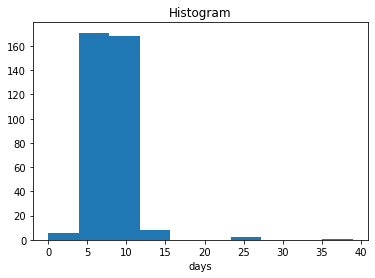
# What's the typical interval between scenes?
good.time.diff("time").dt.days.plot.hist()
[14]:
(array([  6., 171., 168.,   8.,   0.,   0.,   2.,   0.,   0.,   1.]),
 array([ 0. ,  3.9,  7.8, 11.7, 15.6, 19.5, 23.4, 27.3, 31.2, 35.1, 39. ]),
 <BarContainer object of 10 artists>)
Make biannual median composites
The Landsat-8 scenes appear to typically be 5-10 days apart. Let’s composite that down to a 6-month interval.
Since the cloudy pixels we masked with NaNs will be ignored in the median, this should give us a decent cloud-free-ish image for each.
[15]:
# Make biannual median composites (`2Q` means 2 quarters)
composites = good.resample(time="2Q").median("time")
composites
[15]:
<xarray.DataArray 'stackstac-9678efaf932b81b94aa1dceb9a89fb92' (time: 17, band: 19, y: 774, x: 1261)>
dask.array<stack, shape=(17, 19, 774, 1261), dtype=float64, chunksize=(1, 1, 774, 512), chunktype=numpy.ndarray>
Coordinates:
  * time                       (time) datetime64[ns] 2013-03-31 ... 2021-03-31
  * band                       (band) object 'QA_PIXEL' 'QA_RADSAT' ... 'ST_QA'
  * x                          (x) float64 4.024e+05 4.025e+05 ... 4.402e+05
  * y                          (y) float64 4.623e+06 4.623e+06 ... 4.6e+06
    landsat:wrs_type           <U1 '2'
    platform                   <U9 'landsat-8'
    view:off_nadir             int64 0
    landsat:wrs_row            <U3 '031'
    landsat:collection_number  <U2 '02'
    landsat:processing_level   <U4 'L2SP'
    proj:epsg                  int64 32619
instruments object {'oli', 'tirs'}- time: 17
- band: 19
- y: 774
- x: 1261
- dask.array<chunksize=(1, 1, 774, 512), meta=np.ndarray>
Array Chunk Bytes 2.35 GiB 3.02 MiB Shape (17, 19, 774, 1261) (1, 1, 774, 512) Count 74275 Tasks 969 Chunks Type float64 numpy.ndarray - time(time)datetime64[ns]2013-03-31 ... 2021-03-31
array(['2013-03-31T00:00:00.000000000', '2013-09-30T00:00:00.000000000', '2014-03-31T00:00:00.000000000', '2014-09-30T00:00:00.000000000', '2015-03-31T00:00:00.000000000', '2015-09-30T00:00:00.000000000', '2016-03-31T00:00:00.000000000', '2016-09-30T00:00:00.000000000', '2017-03-31T00:00:00.000000000', '2017-09-30T00:00:00.000000000', '2018-03-31T00:00:00.000000000', '2018-09-30T00:00:00.000000000', '2019-03-31T00:00:00.000000000', '2019-09-30T00:00:00.000000000', '2020-03-31T00:00:00.000000000', '2020-09-30T00:00:00.000000000', '2021-03-31T00:00:00.000000000'], dtype='datetime64[ns]') - band(band)object'QA_PIXEL' 'QA_RADSAT' ... 'ST_QA'
array(['QA_PIXEL', 'QA_RADSAT', 'coastal', 'blue', 'green', 'red', 'nir08', 'swir16', 'swir22', 'SR_B8', 'lwir11', 'ST_ATRAN', 'ST_CDIST', 'ST_DRAD', 'ST_URAD', 'ST_TRAD', 'ST_EMIS', 'ST_EMSD', 'ST_QA'], dtype=object) - x(x)float644.024e+05 4.025e+05 ... 4.402e+05
array([402441.341155, 402471.337155, 402501.333156, ..., 440176.309825, 440206.305826, 440236.301826]) - y(y)float644.623e+06 4.623e+06 ... 4.6e+06
array([4622904.475909, 4622874.479936, 4622844.483962, ..., 4599777.580191, 4599747.584217, 4599717.588243]) - landsat:wrs_type()<U1'2'
array('2', dtype='<U1') - platform()<U9'landsat-8'
array('landsat-8', dtype='<U9') - view:off_nadir()int640
array(0)
- landsat:wrs_row()<U3'031'
array('031', dtype='<U3') - landsat:collection_number()<U2'02'
array('02', dtype='<U2') - landsat:processing_level()<U4'L2SP'
array('L2SP', dtype='<U4') - proj:epsg()int6432619
array(32619)
- instruments()object{'oli', 'tirs'}
array({'oli', 'tirs'}, dtype=object)
Pick the red-green-blue bands to make a true-color image.
[16]:
rgb = composites.sel(band=["red", "green", "blue"])
rgb
[16]:
<xarray.DataArray 'stackstac-9678efaf932b81b94aa1dceb9a89fb92' (time: 17, band: 3, y: 774, x: 1261)>
dask.array<getitem, shape=(17, 3, 774, 1261), dtype=float64, chunksize=(1, 1, 774, 512), chunktype=numpy.ndarray>
Coordinates:
  * time                       (time) datetime64[ns] 2013-03-31 ... 2021-03-31
  * band                       (band) object 'red' 'green' 'blue'
  * x                          (x) float64 4.024e+05 4.025e+05 ... 4.402e+05
  * y                          (y) float64 4.623e+06 4.623e+06 ... 4.6e+06
    landsat:wrs_type           <U1 '2'
    platform                   <U9 'landsat-8'
    view:off_nadir             int64 0
    landsat:wrs_row            <U3 '031'
    landsat:collection_number  <U2 '02'
    landsat:processing_level   <U4 'L2SP'
    proj:epsg                  int64 32619
instruments object {'oli', 'tirs'}- time: 17
- band: 3
- y: 774
- x: 1261
- dask.array<chunksize=(1, 1, 774, 512), meta=np.ndarray>
Array Chunk Bytes 379.77 MiB 3.02 MiB Shape (17, 3, 774, 1261) (1, 1, 774, 512) Count 74428 Tasks 153 Chunks Type float64 numpy.ndarray - time(time)datetime64[ns]2013-03-31 ... 2021-03-31
array(['2013-03-31T00:00:00.000000000', '2013-09-30T00:00:00.000000000', '2014-03-31T00:00:00.000000000', '2014-09-30T00:00:00.000000000', '2015-03-31T00:00:00.000000000', '2015-09-30T00:00:00.000000000', '2016-03-31T00:00:00.000000000', '2016-09-30T00:00:00.000000000', '2017-03-31T00:00:00.000000000', '2017-09-30T00:00:00.000000000', '2018-03-31T00:00:00.000000000', '2018-09-30T00:00:00.000000000', '2019-03-31T00:00:00.000000000', '2019-09-30T00:00:00.000000000', '2020-03-31T00:00:00.000000000', '2020-09-30T00:00:00.000000000', '2021-03-31T00:00:00.000000000'], dtype='datetime64[ns]') - band(band)object'red' 'green' 'blue'
array(['red', 'green', 'blue'], dtype=object)
- x(x)float644.024e+05 4.025e+05 ... 4.402e+05
array([402441.341155, 402471.337155, 402501.333156, ..., 440176.309825, 440206.305826, 440236.301826]) - y(y)float644.623e+06 4.623e+06 ... 4.6e+06
array([4622904.475909, 4622874.479936, 4622844.483962, ..., 4599777.580191, 4599747.584217, 4599717.588243]) - landsat:wrs_type()<U1'2'
array('2', dtype='<U1') - platform()<U9'landsat-8'
array('landsat-8', dtype='<U9') - view:off_nadir()int640
array(0)
- landsat:wrs_row()<U3'031'
array('031', dtype='<U3') - landsat:collection_number()<U2'02'
array('02', dtype='<U2') - landsat:processing_level()<U4'L2SP'
array('L2SP', dtype='<U4') - proj:epsg()int6432619
array(32619)
- instruments()object{'oli', 'tirs'}
array({'oli', 'tirs'}, dtype=object)
Some final cleanup to make a nicer-looking animation:
Drop the 2021 dates, since we’re not far enough into 2021 yet to have enough scenes for a nice-looking composite.
Forward-fill any NaN pixels from the previous frame, to make the animation look less jumpy.
Also skip the first frame, since its NaNs can’t be filled from anywhere.
[17]:
cleaned = rgb.loc[:"2021-01-01"].ffill("time")[1:]
Render the GIF
Use GeoGIF to turn the stack into an animation. We’ll use dgif to render the GIF on the cluster, so there’s less data to send back. (GIFs are a lot smaller than NumPy arrays!)
[18]:
%%time
gif_img = geogif.dgif(cleaned).compute()
CPU times: user 2.54 s, sys: 121 ms, total: 2.66 s
Wall time: 25.2 s
[19]:
# we turned ~7GiB of data into a 4MB GIF!
dask.utils.format_bytes(len(gif_img.data))
[19]:
'3.99 MiB'
[20]:
gif_img
[20]: