Note
You can view & download the original notebook on GitHub.
Basic example#
We’ll search for two months of Sentinel-2 data overlapping our area of interest—in this case, the Santa Fe ski area in New Mexico, USA (Google maps).
We use stackstac to create an xarray of all the data. From there, it’s easy to filter out cloudy scenes from the array based on their metadata, then create a median composite for each month.
[1]:
import stackstac
[2]:
lon, lat = -105.78, 35.79
We use pystac-client to find the relevant STAC (Spatio-Temporal Asset Catalog) items. These basically provide metadata about the relevant scenes, and links to their data.
We’ll use element84’s search endpoint to look for items from the sentinel-2-l2a collection on AWS.
[3]:
import pystac_client
URL = "https://earth-search.aws.element84.com/v1"
catalog = pystac_client.Client.open(URL)
[4]:
%%time
items = catalog.search(
    intersects=dict(type="Point", coordinates=[lon, lat]),
    collections=["sentinel-2-l2a"],
    datetime="2020-03-01/2020-06-01"
).item_collection()
len(items)
CPU times: user 107 ms, sys: 17 ms, total: 124 ms
Wall time: 1.27 s
[4]:
42
Use stackstac to turn those STAC items into a lazy xarray. Using all the defaults, our data will be in its native coordinate reference system, at the finest resolution of all the assets.
[5]:
%time stack = stackstac.stack(items)
CPU times: user 115 ms, sys: 3.43 ms, total: 119 ms
Wall time: 117 ms
[6]:
stack
[6]:
<xarray.DataArray 'stackstac-3a21164f19f81366a5242c365d798d31' (time: 42,
                                                                band: 32,
                                                                y: 10980,
                                                                x: 10980)>
dask.array<fetch_raster_window, shape=(42, 32, 10980, 10980), dtype=float64, chunksize=(1, 1, 1024, 1024), chunktype=numpy.ndarray>
Coordinates: (12/52)
  * time                                     (time) datetime64[ns] 2020-03-02...
    id                                       (time) <U24 'S2B_13SDV_20200302_...
  * band                                     (band) <U12 'aot' ... 'wvp-jp2'
  * x                                        (x) float64 4e+05 ... 5.098e+05
  * y                                        (y) float64 4e+06 ... 3.89e+06
    s2:product_type                          <U7 'S2MSI2A'
    ...                                       ...
    raster:bands                             (band) object [{'nodata': 0, 'da...
    gsd                                      (band) object None 10 ... None None
    common_name                              (band) object None 'blue' ... None
    center_wavelength                        (band) object None 0.49 ... None
    full_width_half_max                      (band) object None 0.098 ... None
    epsg                                     int64 32613
Attributes:
    spec:        RasterSpec(epsg=32613, bounds=(399960.0, 3890220.0, 509760.0...
    crs:         epsg:32613
    transform:   | 10.00, 0.00, 399960.00|\n| 0.00,-10.00, 4000020.00|\n| 0.0...
resolution: 10.0- time: 42
- band: 32
- y: 10980
- x: 10980
- dask.array<chunksize=(1, 1, 1024, 1024), meta=np.ndarray>
Array Chunk Bytes 1.18 TiB 8.00 MiB Shape (42, 32, 10980, 10980) (1, 1, 1024, 1024) Dask graph 162624 chunks in 3 graph layers Data type float64 numpy.ndarray - time(time)datetime64[ns]2020-03-02T18:04:04.524000 ... 2...
array(['2020-03-02T18:04:04.524000000', '2020-03-04T17:54:07.095000000', '2020-03-07T18:04:02.946000000', '2020-03-09T17:54:09.291000000', '2020-03-12T18:04:04.983000000', '2020-03-14T17:54:07.621000000', '2020-03-17T18:04:03.272000000', '2020-03-19T17:54:09.361000000', '2020-03-22T18:04:04.927000000', '2020-03-24T17:54:07.643000000', '2020-03-27T18:04:03.119000000', '2020-03-29T17:54:08.945000000', '2020-04-01T18:04:04.327000000', '2020-04-03T17:54:07.524000000', '2020-04-06T18:04:04.095000000', '2020-04-08T17:54:08.005000000', '2020-04-11T18:04:03.225000000', '2020-04-13T17:54:10.480000000', '2020-04-16T18:04:06.843000000', '2020-04-18T17:54:06.501000000', '2020-04-21T18:04:01.588000000', '2020-04-23T17:54:12.962000000', '2020-04-26T18:04:09.127000000', '2020-04-28T17:54:06.998000000', '2020-05-01T18:04:03.406000000', '2020-05-03T17:54:14.877000000', '2020-05-06T18:04:10.877000000', '2020-05-08T17:54:09.389000000', '2020-05-11T18:04:05.599000000', '2020-05-13T17:54:16.280000000', '2020-05-16T18:04:12.105000000', '2020-05-18T17:54:11.240000000', '2020-05-18T17:54:11.240000000', '2020-05-21T18:04:07.312000000', '2020-05-21T18:04:07.313000000', '2020-05-23T17:54:17.223000000', '2020-05-23T17:54:17.224000000', '2020-05-26T18:04:12.901000000', '2020-05-26T18:04:12.903000000', '2020-05-28T17:54:12.637000000', '2020-05-31T18:04:08.524000000', '2020-05-31T18:04:08.524000000'], dtype='datetime64[ns]') - id(time)<U24'S2B_13SDV_20200302_0_L2A' ... '...
array(['S2B_13SDV_20200302_0_L2A', 'S2A_13SDV_20200304_0_L2A', 'S2A_13SDV_20200307_0_L2A', 'S2B_13SDV_20200309_0_L2A', 'S2B_13SDV_20200312_0_L2A', 'S2A_13SDV_20200314_0_L2A', 'S2A_13SDV_20200317_0_L2A', 'S2B_13SDV_20200319_0_L2A', 'S2B_13SDV_20200322_0_L2A', 'S2A_13SDV_20200324_0_L2A', 'S2A_13SDV_20200327_0_L2A', 'S2B_13SDV_20200329_0_L2A', 'S2B_13SDV_20200401_0_L2A', 'S2A_13SDV_20200403_0_L2A', 'S2A_13SDV_20200406_0_L2A', 'S2B_13SDV_20200408_0_L2A', 'S2B_13SDV_20200411_0_L2A', 'S2A_13SDV_20200413_0_L2A', 'S2A_13SDV_20200416_0_L2A', 'S2B_13SDV_20200418_0_L2A', 'S2B_13SDV_20200421_0_L2A', 'S2A_13SDV_20200423_0_L2A', 'S2A_13SDV_20200426_0_L2A', 'S2B_13SDV_20200428_0_L2A', 'S2B_13SDV_20200501_0_L2A', 'S2A_13SDV_20200503_0_L2A', 'S2A_13SDV_20200506_0_L2A', 'S2B_13SDV_20200508_0_L2A', 'S2B_13SDV_20200511_0_L2A', 'S2A_13SDV_20200513_0_L2A', 'S2A_13SDV_20200516_0_L2A', 'S2B_13SDV_20200518_1_L2A', 'S2B_13SDV_20200518_0_L2A', 'S2B_13SDV_20200521_0_L2A', 'S2B_13SDV_20200521_1_L2A', 'S2A_13SDV_20200523_1_L2A', 'S2A_13SDV_20200523_0_L2A', 'S2A_13SDV_20200526_1_L2A', 'S2A_13SDV_20200526_0_L2A', 'S2B_13SDV_20200528_0_L2A', 'S2B_13SDV_20200531_1_L2A', 'S2B_13SDV_20200531_0_L2A'], dtype='<U24') - band(band)<U12'aot' 'blue' ... 'wvp-jp2'
array(['aot', 'blue', 'coastal', 'green', 'nir', 'nir08', 'nir09', 'red', 'rededge1', 'rededge2', 'rededge3', 'scl', 'swir16', 'swir22', 'visual', 'wvp', 'aot-jp2', 'blue-jp2', 'coastal-jp2', 'green-jp2', 'nir-jp2', 'nir08-jp2', 'nir09-jp2', 'red-jp2', 'rededge1-jp2', 'rededge2-jp2', 'rededge3-jp2', 'scl-jp2', 'swir16-jp2', 'swir22-jp2', 'visual-jp2', 'wvp-jp2'], dtype='<U12') - x(x)float644e+05 4e+05 ... 5.097e+05 5.098e+05
array([399960., 399970., 399980., ..., 509730., 509740., 509750.])
- y(y)float644e+06 4e+06 ... 3.89e+06 3.89e+06
array([4000020., 4000010., 4000000., ..., 3890250., 3890240., 3890230.])
- s2:product_type()<U7'S2MSI2A'
array('S2MSI2A', dtype='<U7') - s2:product_uri(time)<U65'S2B_MSIL2A_20200302T175139_N021...
array(['S2B_MSIL2A_20200302T175139_N0214_R141_T13SDV_20200302T215903.SAFE', 'S2A_MSIL2A_20200304T174211_N0214_R098_T13SDV_20200304T215256.SAFE', 'S2A_MSIL2A_20200307T175151_N0214_R141_T13SDV_20200307T224018.SAFE', 'S2B_MSIL2A_20200309T174049_N0214_R098_T13SDV_20200309T222757.SAFE', 'S2B_MSIL2A_20200312T175029_N0214_R141_T13SDV_20200312T220221.SAFE', 'S2A_MSIL2A_20200314T174101_N0214_R098_T13SDV_20200314T220229.SAFE', 'S2A_MSIL2A_20200317T175041_N0214_R141_T13SDV_20200317T220112.SAFE', 'S2B_MSIL2A_20200319T173929_N0214_R098_T13SDV_20200319T222046.SAFE', 'S2B_MSIL2A_20200322T174919_N0214_R141_T13SDV_20200322T214308.SAFE', 'S2A_MSIL2A_20200324T173951_N0214_R098_T13SDV_20200324T220044.SAFE', 'S2A_MSIL2A_20200327T174941_N0214_R141_T13SDV_20200327T221015.SAFE', 'S2B_MSIL2A_20200329T173859_N0214_R098_T13SDV_20200329T222636.SAFE', 'S2B_MSIL2A_20200401T174909_N0214_R141_T13SDV_20200401T220155.SAFE', 'S2A_MSIL2A_20200403T173901_N0214_R098_T13SDV_20200403T220105.SAFE', 'S2A_MSIL2A_20200406T174901_N0214_R141_T13SDV_20200406T221027.SAFE', 'S2B_MSIL2A_20200408T173859_N0214_R098_T13SDV_20200408T215856.SAFE', 'S2B_MSIL2A_20200411T174909_N0214_R141_T13SDV_20200411T220443.SAFE', 'S2A_MSIL2A_20200413T173901_N0214_R098_T13SDV_20200413T235616.SAFE', 'S2A_MSIL2A_20200416T174911_N0214_R141_T13SDV_20200416T221101.SAFE', 'S2B_MSIL2A_20200418T173859_N0214_R098_T13SDV_20200418T214953.SAFE', ... 'S2B_MSIL2A_20200428T173859_N0214_R098_T13SDV_20200428T214309.SAFE', 'S2B_MSIL2A_20200501T174909_N0214_R141_T13SDV_20200501T220131.SAFE', 'S2A_MSIL2A_20200503T173911_N0214_R098_T13SDV_20200503T220129.SAFE', 'S2A_MSIL2A_20200506T174911_N0214_R141_T13SDV_20200506T235226.SAFE', 'S2B_MSIL2A_20200508T173859_N0214_R098_T13SDV_20200508T215220.SAFE', 'S2B_MSIL2A_20200511T174909_N0214_R141_T13SDV_20200511T220228.SAFE', 'S2A_MSIL2A_20200513T173911_N0214_R098_T13SDV_20200513T220059.SAFE', 'S2A_MSIL2A_20200516T174911_N0214_R141_T13SDV_20200516T220523.SAFE', 'S2B_MSIL2A_20200518T173909_N0500_R098_T13SDV_20230506T114618.SAFE', 'S2B_MSIL2A_20200518T173909_N0214_R098_T13SDV_20200518T214934.SAFE', 'S2B_MSIL2A_20200521T174909_N0214_R141_T13SDV_20200521T214346.SAFE', 'S2B_MSIL2A_20200521T174909_N0500_R141_T13SDV_20230414T012336.SAFE', 'S2A_MSIL2A_20200523T173911_N0500_R098_T13SDV_20230412T234513.SAFE', 'S2A_MSIL2A_20200523T173911_N0214_R098_T13SDV_20200523T233334.SAFE', 'S2A_MSIL2A_20200526T174911_N0500_R141_T13SDV_20230415T205610.SAFE', 'S2A_MSIL2A_20200526T174911_N0214_R141_T13SDV_20200526T220745.SAFE', 'S2B_MSIL2A_20200528T173909_N0214_R098_T13SDV_20200528T213421.SAFE', 'S2B_MSIL2A_20200531T174909_N0500_R141_T13SDV_20230509T035228.SAFE', 'S2B_MSIL2A_20200531T174909_N0214_R141_T13SDV_20200531T220418.SAFE'], dtype='<U65') - s2:dark_features_percentage(time)object5.964193 0.977774 ... 0.548386
array([5.964193, 0.977774, 3.818965, 1.609308, 5.547048, 1.798176, 0, 3.328483, 0, 0.33615, 2.725101, 1.753066, 4.251513, 0.411445, 1.884744, 0.47257, 1.734854, 0, 2.026237, 3.005747, 7.286789, 0.67667, 0.00177, 0.136615, 2.092979, 0.057468, 0.982041, 0.456389, 0.005127, 0.236887, 0.55769, 0.007674, 0.024117, 0.311602, 0.456542, 0.01133, 0.037226, 0.473004, 0.345139, 2.483595, 0.217085, 0.548386], dtype=object) - earthsearch:payload_id(time)<U74'roda-sentinel2/workflow-sentine...
array(['roda-sentinel2/workflow-sentinel2-to-stac/961c597ba6dbc41345a2528cde2a8aec', 'roda-sentinel2/workflow-sentinel2-to-stac/e624ac5bd03f6d246fd370a92fe2c162', 'roda-sentinel2/workflow-sentinel2-to-stac/4670cb0b678fed100abded0989c3d546', 'roda-sentinel2/workflow-sentinel2-to-stac/437c5bf62f2f45c1348b7f9f6c6a40a4', 'roda-sentinel2/workflow-sentinel2-to-stac/0f750d33cb08ac2440064369bf3b716d', 'roda-sentinel2/workflow-sentinel2-to-stac/dc03d6335d4d32dfd3b3685b9e3e0d24', 'roda-sentinel2/workflow-sentinel2-to-stac/db8dfbfa901a321cd9feb7ff15576f54', 'roda-sentinel2/workflow-sentinel2-to-stac/94a1cba9235251183fffd2454f92e18d', 'roda-sentinel2/workflow-sentinel2-to-stac/6878668e00874dc7edf9ef79ad40d873', 'roda-sentinel2/workflow-sentinel2-to-stac/22b34e8df1097f3dc4310e0c760e93f5', 'roda-sentinel2/workflow-sentinel2-to-stac/4b4d48a1a5a4bf8e85a9fc4bcde74ba1', 'roda-sentinel2/workflow-sentinel2-to-stac/13a12ebaafb2efc5854d98f7a0b96994', 'roda-sentinel2/workflow-sentinel2-to-stac/afb43c585d466972865ed5139ba35520', 'roda-sentinel2/workflow-sentinel2-to-stac/00bfe5eff22b9aae0b5adfae696a11fa', 'roda-sentinel2/workflow-sentinel2-to-stac/2758e5e900c1639f19b11efe3fbbbc26', 'roda-sentinel2/workflow-sentinel2-to-stac/861d7837603c47c9badccf7641222c43', 'roda-sentinel2/workflow-sentinel2-to-stac/d00c2b2ec66eb2ee26e3c9c77c92924d', 'roda-sentinel2/workflow-sentinel2-to-stac/f1e8d6da18b30cec574888940cda178d', 'roda-sentinel2/workflow-sentinel2-to-stac/4b9a452ca3ca22eb3d47d2b5355a4b58', 'roda-sentinel2/workflow-sentinel2-to-stac/b9fc7bcdb051f480f06de7e2c2689f18', ... 'roda-sentinel2/workflow-sentinel2-to-stac/5da6662d888f5a2c239f2a42fc906e16', 'roda-sentinel2/workflow-sentinel2-to-stac/8cb780dd6c214e106af6a6923a35f5db', 'roda-sentinel2/workflow-sentinel2-to-stac/940326327617d4347302465474ee13fb', 'roda-sentinel2/workflow-sentinel2-to-stac/d1bd3ffa19dcaeac635edefff4c1d085', 'roda-sentinel2/workflow-sentinel2-to-stac/8a247297d956ce82fd7c76380d91013a', 'roda-sentinel2/workflow-sentinel2-to-stac/012117d39c62e03d61d3a9f2c159f0b2', 'roda-sentinel2/workflow-sentinel2-to-stac/68ff35dac2b2aa306e7a3946298a3ba2', 'roda-sentinel2/workflow-sentinel2-to-stac/0d588ed1a8452a3fa426e0be1b2092ae', 'roda-sentinel2/workflow-sentinel2-to-stac/e13e95e89996259eb2f8df605acfd605', 'roda-sentinel2/workflow-sentinel2-to-stac/c73881b42124259ffc57704a24fea2a9', 'roda-sentinel2/workflow-sentinel2-to-stac/bf7badcade62a24d1b1138936f31c334', 'roda-sentinel2/workflow-sentinel2-to-stac/d25cd49f1149d5a144b4ae2dc2eae17b', 'roda-sentinel2/workflow-sentinel2-to-stac/0ae1fe1754605fc2803110991f55ddc4', 'roda-sentinel2/workflow-sentinel2-to-stac/63e96142ca6351d8ac4ef8268aeec4d2', 'roda-sentinel2/workflow-sentinel2-to-stac/ed04bcf83e8e777a4ad64acfe275a73a', 'roda-sentinel2/workflow-sentinel2-to-stac/f2639dd1ea6061226ac0afd6c3dbdc44', 'roda-sentinel2/workflow-sentinel2-to-stac/adc843839954b0f86e33fc757bc604b7', 'roda-sentinel2/workflow-sentinel2-to-stac/47cc34f1fcd5b9d0d879aa7302c8cf9a', 'roda-sentinel2/workflow-sentinel2-to-stac/309ccf10b8946d7b537ea389f31e31de'], dtype='<U74') - view:sun_azimuth(time)float64155.3 151.8 154.7 ... 134.5 134.5
array([155.31639429, 151.83197133, 154.73650057, 151.16128803, 154.179699 , 150.45736002, 153.58979378, 149.74608923, 152.99455219, 148.97431657, 152.33929786, 148.16764008, 151.65028202, 147.27598521, 150.88270509, 146.31202768, 150.01908475, 145.2568735 , 149.07574674, 144.02972799, 147.92731169, 142.74214235, 146.73723803, 141.21544202, 145.27949632, 139.65732744, 143.78674097, 137.86113138, 142.03137488, 136.0564562 , 140.26342327, 134.07969866, 134.07751989, 138.30650682, 138.30902048, 132.17656288, 132.17437653, 136.4391216 , 136.43659935, 130.23661127, 134.5383766 , 134.53585544]) - s2:water_percentage(time)object0.065741 0.093663 ... 0.005841
array([0.065741, 0.093663, 0.075816, 0.101901, 0.035346, 0.114024, 0, 0.148254, 0, 0.093507, 0.054821, 0.034439, 0.045153, 0.093679, 0.022672, 0.178901, 0.023153, 0, 0.057075, 0.133032, 0.083357, 0.021841, 0, 0.081463, 0.021284, 0.086221, 0.020722, 0.084598, 0, 0.083805, 0.017448, 0.086994, 0.084406, 0.016444, 0.019862, 0.053855, 0.048278, 0.01961, 0.01413, 0.070995, 0.005737, 0.005841], dtype=object) - s2:sequence(time)<U1'0' '0' '0' '0' ... '0' '0' '1' '0'
array(['0', '0', '0', '0', '0', '0', '0', '0', '0', '0', '0', '0', '0', '0', '0', '0', '0', '0', '0', '0', '0', '0', '0', '0', '0', '0', '0', '0', '0', '0', '0', '1', '0', '0', '1', '1', '0', '1', '0', '0', '1', '0'], dtype='<U1') - constellation()<U10'sentinel-2'
array('sentinel-2', dtype='<U10') - mgrs:grid_square()<U2'DV'
array('DV', dtype='<U2') - s2:high_proba_clouds_percentage(time)object2.049168 0.065789 ... 50.653559
array([2.049168, 0.065789, 0.254371, 1.091201, 10.288216, 1.780565, 69.306839, 45.398596, 14.409222, 0.038636, 49.134019, 14.53899, 20.020688, 0.185381, 0.017221, 0.965886, 0.086335, 11.555343, 3.783941, 23.597032, 15.914457, 15.820621, 33.610359, 0.481458, 0.217096, 0.038845, 0.034627, 0.222448, 72.732186, 0.184843, 0.058061, 1.7e-05, 0.036712, 0.063442, 0, 3.150467, 3.232872, 0.016048, 0.043209, 18.319401, 51.032454, 50.653559], dtype=object) - earthsearch:s3_path(time)<U79's3://sentinel-cogs/sentinel-s2-...
array(['s3://sentinel-cogs/sentinel-s2-l2a-cogs/13/S/DV/2020/3/S2B_13SDV_20200302_0_L2A', 's3://sentinel-cogs/sentinel-s2-l2a-cogs/13/S/DV/2020/3/S2A_13SDV_20200304_0_L2A', 's3://sentinel-cogs/sentinel-s2-l2a-cogs/13/S/DV/2020/3/S2A_13SDV_20200307_0_L2A', 's3://sentinel-cogs/sentinel-s2-l2a-cogs/13/S/DV/2020/3/S2B_13SDV_20200309_0_L2A', 's3://sentinel-cogs/sentinel-s2-l2a-cogs/13/S/DV/2020/3/S2B_13SDV_20200312_0_L2A', 's3://sentinel-cogs/sentinel-s2-l2a-cogs/13/S/DV/2020/3/S2A_13SDV_20200314_0_L2A', 's3://sentinel-cogs/sentinel-s2-l2a-cogs/13/S/DV/2020/3/S2A_13SDV_20200317_0_L2A', 's3://sentinel-cogs/sentinel-s2-l2a-cogs/13/S/DV/2020/3/S2B_13SDV_20200319_0_L2A', 's3://sentinel-cogs/sentinel-s2-l2a-cogs/13/S/DV/2020/3/S2B_13SDV_20200322_0_L2A', 's3://sentinel-cogs/sentinel-s2-l2a-cogs/13/S/DV/2020/3/S2A_13SDV_20200324_0_L2A', 's3://sentinel-cogs/sentinel-s2-l2a-cogs/13/S/DV/2020/3/S2A_13SDV_20200327_0_L2A', 's3://sentinel-cogs/sentinel-s2-l2a-cogs/13/S/DV/2020/3/S2B_13SDV_20200329_0_L2A', 's3://sentinel-cogs/sentinel-s2-l2a-cogs/13/S/DV/2020/4/S2B_13SDV_20200401_0_L2A', 's3://sentinel-cogs/sentinel-s2-l2a-cogs/13/S/DV/2020/4/S2A_13SDV_20200403_0_L2A', 's3://sentinel-cogs/sentinel-s2-l2a-cogs/13/S/DV/2020/4/S2A_13SDV_20200406_0_L2A', 's3://sentinel-cogs/sentinel-s2-l2a-cogs/13/S/DV/2020/4/S2B_13SDV_20200408_0_L2A', 's3://sentinel-cogs/sentinel-s2-l2a-cogs/13/S/DV/2020/4/S2B_13SDV_20200411_0_L2A', 's3://sentinel-cogs/sentinel-s2-l2a-cogs/13/S/DV/2020/4/S2A_13SDV_20200413_0_L2A', 's3://sentinel-cogs/sentinel-s2-l2a-cogs/13/S/DV/2020/4/S2A_13SDV_20200416_0_L2A', 's3://sentinel-cogs/sentinel-s2-l2a-cogs/13/S/DV/2020/4/S2B_13SDV_20200418_0_L2A', ... 's3://sentinel-cogs/sentinel-s2-l2a-cogs/13/S/DV/2020/4/S2B_13SDV_20200428_0_L2A', 's3://sentinel-cogs/sentinel-s2-l2a-cogs/13/S/DV/2020/5/S2B_13SDV_20200501_0_L2A', 's3://sentinel-cogs/sentinel-s2-l2a-cogs/13/S/DV/2020/5/S2A_13SDV_20200503_0_L2A', 's3://sentinel-cogs/sentinel-s2-l2a-cogs/13/S/DV/2020/5/S2A_13SDV_20200506_0_L2A', 's3://sentinel-cogs/sentinel-s2-l2a-cogs/13/S/DV/2020/5/S2B_13SDV_20200508_0_L2A', 's3://sentinel-cogs/sentinel-s2-l2a-cogs/13/S/DV/2020/5/S2B_13SDV_20200511_0_L2A', 's3://sentinel-cogs/sentinel-s2-l2a-cogs/13/S/DV/2020/5/S2A_13SDV_20200513_0_L2A', 's3://sentinel-cogs/sentinel-s2-l2a-cogs/13/S/DV/2020/5/S2A_13SDV_20200516_0_L2A', 's3://sentinel-cogs/sentinel-s2-l2a-cogs/13/S/DV/2020/5/S2B_13SDV_20200518_1_L2A', 's3://sentinel-cogs/sentinel-s2-l2a-cogs/13/S/DV/2020/5/S2B_13SDV_20200518_0_L2A', 's3://sentinel-cogs/sentinel-s2-l2a-cogs/13/S/DV/2020/5/S2B_13SDV_20200521_0_L2A', 's3://sentinel-cogs/sentinel-s2-l2a-cogs/13/S/DV/2020/5/S2B_13SDV_20200521_1_L2A', 's3://sentinel-cogs/sentinel-s2-l2a-cogs/13/S/DV/2020/5/S2A_13SDV_20200523_1_L2A', 's3://sentinel-cogs/sentinel-s2-l2a-cogs/13/S/DV/2020/5/S2A_13SDV_20200523_0_L2A', 's3://sentinel-cogs/sentinel-s2-l2a-cogs/13/S/DV/2020/5/S2A_13SDV_20200526_1_L2A', 's3://sentinel-cogs/sentinel-s2-l2a-cogs/13/S/DV/2020/5/S2A_13SDV_20200526_0_L2A', 's3://sentinel-cogs/sentinel-s2-l2a-cogs/13/S/DV/2020/5/S2B_13SDV_20200528_0_L2A', 's3://sentinel-cogs/sentinel-s2-l2a-cogs/13/S/DV/2020/5/S2B_13SDV_20200531_1_L2A', 's3://sentinel-cogs/sentinel-s2-l2a-cogs/13/S/DV/2020/5/S2B_13SDV_20200531_0_L2A'], dtype='<U79') - s2:vegetation_percentage(time)object6.379609 11.904366 ... 1.734599
array([6.379609, 11.904366, 7.742561, 12.67074, 2.317653, 4.969456, 0, 0.427716, 0, 13.906454, 0.607537, 1.218294, 6.331863, 13.711172, 12.844732, 13.592032, 13.822255, 0, 6.911097, 10.42328, 9.056396, 13.381259, 0.000402, 1.203473, 15.709554, 15.934499, 17.829461, 12.750416, 0, 18.054068, 23.011161, 22.10284, 22.105886, 26.153195, 25.8811, 20.238064, 20.239273, 26.383844, 26.550031, 8.672822, 1.703783, 1.734599], dtype=object) - s2:granule_id(time)<U62'S2B_OPER_MSI_L2A_TL_EPAE_202003...
array(['S2B_OPER_MSI_L2A_TL_EPAE_20200302T215903_A015611_T13SDV_N02.14', 'S2A_OPER_MSI_L2A_TL_SGS__20200304T215256_A024548_T13SDV_N02.14', 'S2A_OPER_MSI_L2A_TL_MTI__20200307T224018_A024591_T13SDV_N02.14', 'S2B_OPER_MSI_L2A_TL_MTI__20200309T222757_A015711_T13SDV_N02.14', 'S2B_OPER_MSI_L2A_TL_EPAE_20200312T220221_A015754_T13SDV_N02.14', 'S2A_OPER_MSI_L2A_TL_SGS__20200314T220229_A024691_T13SDV_N02.14', 'S2A_OPER_MSI_L2A_TL_SGS__20200317T220112_A024734_T13SDV_N02.14', 'S2B_OPER_MSI_L2A_TL_MTI__20200319T222046_A015854_T13SDV_N02.14', 'S2B_OPER_MSI_L2A_TL_EPAE_20200322T214308_A015897_T13SDV_N02.14', 'S2A_OPER_MSI_L2A_TL_SGS__20200324T220044_A024834_T13SDV_N02.14', 'S2A_OPER_MSI_L2A_TL_SGS__20200327T221015_A024877_T13SDV_N02.14', 'S2B_OPER_MSI_L2A_TL_MTI__20200329T222636_A015997_T13SDV_N02.14', 'S2B_OPER_MSI_L2A_TL_EPAE_20200401T220155_A016040_T13SDV_N02.14', 'S2A_OPER_MSI_L2A_TL_SGS__20200403T220105_A024977_T13SDV_N02.14', 'S2A_OPER_MSI_L2A_TL_SGS__20200406T221027_A025020_T13SDV_N02.14', 'S2B_OPER_MSI_L2A_TL_SGS__20200408T215856_A016140_T13SDV_N02.14', 'S2B_OPER_MSI_L2A_TL_EPAE_20200411T220443_A016183_T13SDV_N02.14', 'S2A_OPER_MSI_L2A_TL_MPS__20200413T235616_A025120_T13SDV_N02.14', 'S2A_OPER_MSI_L2A_TL_SGS__20200416T221101_A025163_T13SDV_N02.14', 'S2B_OPER_MSI_L2A_TL_EPAE_20200418T214953_A016283_T13SDV_N02.14', ... 'S2B_OPER_MSI_L2A_TL_EPAE_20200428T214309_A016426_T13SDV_N02.14', 'S2B_OPER_MSI_L2A_TL_EPAE_20200501T220131_A016469_T13SDV_N02.14', 'S2A_OPER_MSI_L2A_TL_SGS__20200503T220129_A025406_T13SDV_N02.14', 'S2A_OPER_MSI_L2A_TL_SGS__20200506T235226_A025449_T13SDV_N02.14', 'S2B_OPER_MSI_L2A_TL_EPAE_20200508T215220_A016569_T13SDV_N02.14', 'S2B_OPER_MSI_L2A_TL_EPAE_20200511T220228_A016612_T13SDV_N02.14', 'S2A_OPER_MSI_L2A_TL_SGS__20200513T220059_A025549_T13SDV_N02.14', 'S2A_OPER_MSI_L2A_TL_SGS__20200516T220523_A025592_T13SDV_N02.14', 'S2B_OPER_MSI_L2A_TL_S2RP_20230506T114618_A016712_T13SDV_N05.00', 'S2B_OPER_MSI_L2A_TL_EPAE_20200518T214934_A016712_T13SDV_N02.14', 'S2B_OPER_MSI_L2A_TL_EPAE_20200521T214346_A016755_T13SDV_N02.14', 'S2B_OPER_MSI_L2A_TL_S2RP_20230414T012336_A016755_T13SDV_N05.00', 'S2A_OPER_MSI_L2A_TL_S2RP_20230412T234513_A025692_T13SDV_N05.00', 'S2A_OPER_MSI_L2A_TL_MPS__20200523T233334_A025692_T13SDV_N02.14', 'S2A_OPER_MSI_L2A_TL_S2RP_20230415T205610_A025735_T13SDV_N05.00', 'S2A_OPER_MSI_L2A_TL_SGS__20200526T220745_A025735_T13SDV_N02.14', 'S2B_OPER_MSI_L2A_TL_EPAE_20200528T213421_A016855_T13SDV_N02.14', 'S2B_OPER_MSI_L2A_TL_S2RP_20230509T035228_A016898_T13SDV_N05.00', 'S2B_OPER_MSI_L2A_TL_EPAE_20200531T220418_A016898_T13SDV_N02.14'], dtype='<U62') - s2:medium_proba_clouds_percentage(time)float644.931 4.147 0.5657 ... 35.23 32.0
array([4.9311680e+00, 4.1468040e+00, 5.6573900e-01, 3.2011840e+00, 2.3123996e+01, 2.8804390e+00, 3.0690882e+01, 1.7411864e+01, 8.5448873e+01, 1.0379200e+00, 1.1961268e+01, 2.4275507e+01, 6.0106470e+00, 7.6067800e-01, 2.2273350e+00, 7.3864700e-01, 1.6059600e-01, 8.5272765e+01, 2.3278300e+00, 9.2296650e+00, 4.9400530e+00, 8.9391280e+00, 5.7952380e+01, 2.8663146e+01, 2.6776270e+00, 5.0180000e-01, 1.5719500e-01, 2.5610470e+00, 2.6468298e+01, 2.6560860e+00, 7.2951000e-02, 4.4800000e-04, 1.2582200e-01, 4.0986000e-02, 4.0700000e-04, 2.7519350e+00, 1.3240139e+01, 4.5534000e-02, 9.2031000e-02, 2.7796990e+00, 3.5225174e+01, 3.1999114e+01]) - grid:code()<U10'MGRS-13SDV'
array('MGRS-13SDV', dtype='<U10') - eo:cloud_cover(time)float646.98 4.213 0.8201 ... 86.26 82.65
array([6.9803360e+00, 4.2125940e+00, 8.2011000e-01, 4.2923840e+00, 3.3412212e+01, 4.6610040e+00, 9.9997720e+01, 6.2810460e+01, 9.9858095e+01, 1.0765560e+00, 6.1095287e+01, 3.8814497e+01, 2.6031335e+01, 9.4605900e-01, 2.2445570e+00, 1.7045330e+00, 2.4693100e-01, 9.6828108e+01, 6.1117700e+00, 3.2826912e+01, 2.0854510e+01, 2.4759749e+01, 9.1562739e+01, 2.9144605e+01, 2.8947240e+00, 5.4064500e-01, 1.9182200e-01, 2.7834940e+00, 9.9200484e+01, 2.8409300e+00, 1.3101200e-01, 4.6400000e-04, 1.6253400e-01, 1.0442800e-01, 4.0700000e-04, 5.9024020e+00, 1.6473012e+01, 6.1582000e-02, 1.3524000e-01, 2.1099100e+01, 8.6257631e+01, 8.2652673e+01]) - s2:processing_baseline(time)<U5'02.14' '02.14' ... '05.00' '02.14'
array(['02.14', '02.14', '02.14', '02.14', '02.14', '02.14', '02.14', '02.14', '02.14', '02.14', '02.14', '02.14', '02.14', '02.14', '02.14', '02.14', '02.14', '02.14', '02.14', '02.14', '02.14', '02.14', '02.14', '02.14', '02.14', '02.14', '02.14', '02.14', '02.14', '02.14', '02.14', '05.00', '02.14', '02.14', '05.00', '05.00', '02.14', '05.00', '02.14', '02.14', '05.00', '02.14'], dtype='<U5') - earthsearch:boa_offset_applied(time)boolFalse False False ... True False
array([False, False, False, False, False, False, False, False, False, False, False, False, False, False, False, False, False, False, False, False, False, False, False, False, False, False, False, False, False, False, False, True, False, False, True, True, False, True, False, False, True, False]) - proj:epsg()int6432613
array(32613)
- s2:datastrip_id(time)<U64'S2B_OPER_MSI_L2A_DS_EPAE_202003...
array(['S2B_OPER_MSI_L2A_DS_EPAE_20200302T215903_S20200302T180242_N02.14', 'S2A_OPER_MSI_L2A_DS_SGS__20200304T215256_S20200304T175215_N02.14', 'S2A_OPER_MSI_L2A_DS_MTI__20200307T224018_S20200307T175330_N02.14', 'S2B_OPER_MSI_L2A_DS_MTI__20200309T222757_S20200309T174619_N02.14', 'S2B_OPER_MSI_L2A_DS_EPAE_20200312T220221_S20200312T175859_N02.14', 'S2A_OPER_MSI_L2A_DS_SGS__20200314T220229_S20200314T174952_N02.14', 'S2A_OPER_MSI_L2A_DS_SGS__20200317T220112_S20200317T180336_N02.14', 'S2B_OPER_MSI_L2A_DS_MTI__20200319T222046_S20200319T174930_N02.14', 'S2B_OPER_MSI_L2A_DS_EPAE_20200322T214308_S20200322T175638_N02.14', 'S2A_OPER_MSI_L2A_DS_SGS__20200324T220044_S20200324T174741_N02.14', 'S2A_OPER_MSI_L2A_DS_SGS__20200327T221015_S20200327T175756_N02.14', 'S2B_OPER_MSI_L2A_DS_MTI__20200329T222636_S20200329T174617_N02.14', 'S2B_OPER_MSI_L2A_DS_EPAE_20200401T220155_S20200401T175716_N02.14', 'S2A_OPER_MSI_L2A_DS_SGS__20200403T220105_S20200403T174815_N02.14', 'S2A_OPER_MSI_L2A_DS_SGS__20200406T221027_S20200406T175657_N02.14', 'S2B_OPER_MSI_L2A_DS_SGS__20200408T215856_S20200408T174547_N02.14', 'S2B_OPER_MSI_L2A_DS_EPAE_20200411T220443_S20200411T175522_N02.14', 'S2A_OPER_MSI_L2A_DS_MPS__20200413T235616_S20200413T174358_N02.14', 'S2A_OPER_MSI_L2A_DS_SGS__20200416T221101_S20200416T175652_N02.14', 'S2B_OPER_MSI_L2A_DS_EPAE_20200418T214953_S20200418T174311_N02.14', ... 'S2B_OPER_MSI_L2A_DS_EPAE_20200428T214309_S20200428T174651_N02.14', 'S2B_OPER_MSI_L2A_DS_EPAE_20200501T220131_S20200501T175736_N02.14', 'S2A_OPER_MSI_L2A_DS_SGS__20200503T220129_S20200503T174634_N02.14', 'S2A_OPER_MSI_L2A_DS_SGS__20200506T235226_S20200506T175505_N02.14', 'S2B_OPER_MSI_L2A_DS_EPAE_20200508T215220_S20200508T174740_N02.14', 'S2B_OPER_MSI_L2A_DS_EPAE_20200511T220228_S20200511T175546_N02.14', 'S2A_OPER_MSI_L2A_DS_SGS__20200513T220059_S20200513T174559_N02.14', 'S2A_OPER_MSI_L2A_DS_SGS__20200516T220523_S20200516T175955_N02.14', 'S2B_OPER_MSI_L2A_DS_S2RP_20230506T114618_S20200518T174525_N05.00', 'S2B_OPER_MSI_L2A_DS_EPAE_20200518T214934_S20200518T174525_N02.14', 'S2B_OPER_MSI_L2A_DS_EPAE_20200521T214346_S20200521T175736_N02.14', 'S2B_OPER_MSI_L2A_DS_S2RP_20230414T012336_S20200521T175736_N05.00', 'S2A_OPER_MSI_L2A_DS_S2RP_20230412T234513_S20200523T175255_N05.00', 'S2A_OPER_MSI_L2A_DS_MPS__20200523T233334_S20200523T175255_N02.14', 'S2A_OPER_MSI_L2A_DS_S2RP_20230415T205610_S20200526T175955_N05.00', 'S2A_OPER_MSI_L2A_DS_SGS__20200526T220745_S20200526T175955_N02.14', 'S2B_OPER_MSI_L2A_DS_EPAE_20200528T213421_S20200528T174743_N02.14', 'S2B_OPER_MSI_L2A_DS_S2RP_20230509T035228_S20200531T175738_N05.00', 'S2B_OPER_MSI_L2A_DS_EPAE_20200531T220418_S20200531T175738_N02.14'], dtype='<U64') - created(time)<U24'2022-11-06T07:24:21.287Z' ... '...
array(['2022-11-06T07:24:21.287Z', '2022-11-06T07:33:23.048Z', '2022-11-06T10:18:48.602Z', '2022-11-03T20:40:01.875Z', '2022-11-06T14:31:12.944Z', '2022-11-06T14:31:19.130Z', '2022-11-06T07:24:31.803Z', '2022-11-06T07:24:50.433Z', '2022-11-06T07:24:23.711Z', '2022-11-06T14:31:13.727Z', '2022-11-06T14:31:16.658Z', '2022-11-06T07:34:37.431Z', '2022-11-06T10:14:16.681Z', '2022-11-06T07:21:36.990Z', '2022-11-06T10:14:20.981Z', '2022-11-06T10:14:26.677Z', '2022-11-06T10:14:16.074Z', '2022-11-06T07:27:18.650Z', '2022-11-06T07:27:11.554Z', '2022-11-06T07:24:56.685Z', '2022-11-06T07:24:56.556Z', '2022-11-06T07:23:13.130Z', '2022-11-06T07:23:23.160Z', '2022-11-06T07:21:17.263Z', '2022-11-06T07:22:17.425Z', '2022-11-06T10:07:56.562Z', '2022-11-06T10:09:23.999Z', '2022-11-06T14:58:38.497Z', '2022-11-06T07:22:22.158Z', '2022-11-06T10:15:17.143Z', '2022-11-06T10:15:11.515Z', '2023-09-19T17:39:04.727Z', '2022-11-06T07:25:19.838Z', '2022-11-06T07:25:12.870Z', '2023-09-19T01:26:11.344Z', '2023-09-17T16:45:47.308Z', '2022-11-06T07:23:56.776Z', '2023-09-16T19:54:01.034Z', '2022-11-06T07:23:57.069Z', '2022-11-06T10:07:59.797Z', '2023-09-15T08:40:04.164Z', '2022-11-06T10:09:18.386Z'], dtype='<U24') - platform(time)<U11'sentinel-2b' ... 'sentinel-2b'
array(['sentinel-2b', 'sentinel-2a', 'sentinel-2a', 'sentinel-2b', 'sentinel-2b', 'sentinel-2a', 'sentinel-2a', 'sentinel-2b', 'sentinel-2b', 'sentinel-2a', 'sentinel-2a', 'sentinel-2b', 'sentinel-2b', 'sentinel-2a', 'sentinel-2a', 'sentinel-2b', 'sentinel-2b', 'sentinel-2a', 'sentinel-2a', 'sentinel-2b', 'sentinel-2b', 'sentinel-2a', 'sentinel-2a', 'sentinel-2b', 'sentinel-2b', 'sentinel-2a', 'sentinel-2a', 'sentinel-2b', 'sentinel-2b', 'sentinel-2a', 'sentinel-2a', 'sentinel-2b', 'sentinel-2b', 'sentinel-2b', 'sentinel-2b', 'sentinel-2a', 'sentinel-2a', 'sentinel-2a', 'sentinel-2a', 'sentinel-2b', 'sentinel-2b', 'sentinel-2b'], dtype='<U11') - s2:not_vegetated_percentage(time)object58.237725 69.964749 ... 10.468978
array([58.237725, 69.964749, 67.999941, 69.886857, 47.125068, 59.953725, 0.000596, 22.444773, 0.066957, 75.588524, 26.301509, 41.711113, 53.858513, 77.119505, 72.610897, 78.381914, 75.565374, 0, 67.843735, 46.9926, 52.053899, 55.559385, 7.148998, 66.284305, 73.988646, 80.906683, 77.82467, 81.510013, 0.67972, 77.63136, 74.810016, 77.492762, 77.100772, 72.611809, 73.130238, 71.858096, 62.467003, 72.438776, 71.809936, 64.78042, 8.694656, 10.468978], dtype=object) - s2:unclassified_percentage(time)float6411.21 5.993 8.904 ... 3.114 4.536
array([1.1210359e+01, 5.9930030e+00, 8.9038710e+00, 5.8048050e+00, 8.1154180e+00, 9.0079430e+00, 1.6810000e-03, 6.1463560e+00, 7.4853000e-02, 3.2794950e+00, 4.2476260e+00, 1.3204080e+01, 5.4039110e+00, 2.8782250e+00, 3.9530600e+00, 2.3256760e+00, 3.4695410e+00, 2.4600000e-04, 8.7602840e+00, 3.6643480e+00, 4.8959710e+00, 2.8737300e+00, 9.4503400e-01, 2.9370080e+00, 3.0445820e+00, 1.4809310e+00, 1.8897530e+00, 1.9197610e+00, 1.1466700e-01, 7.8765800e-01, 9.6784700e-01, 1.2833000e-02, 3.4736100e-01, 5.2424700e-01, 7.6581000e-02, 1.7134120e+00, 6.3813300e-01, 1.3575200e-01, 7.7327100e-01, 1.7892410e+00, 3.1142480e+00, 4.5362630e+00]) - s2:degraded_msi_data_percentage(time)object0 0 0 0 0 0 ... 0.0008 0 0 0.8013 0
array([0, 0, 0, 0, 0, 0, 0, 0, 0, 0, 0, 0, 0, 0, 0, 0, 0, 0, 0, 0, 0, 0, 0, 0, 0, 0, 0, 0, 0, 0, 0, 0.0106, 0, 0, 0.0163, 0, 0, 0.0008, 0, 0, 0.8013, 0], dtype=object) - view:sun_elevation(time)float6444.46 44.31 46.37 ... 71.79 71.78
array([44.46109457, 44.31201576, 46.37271632, 46.22587533, 48.32531762, 48.16279958, 50.29251296, 50.1185939 , 52.2688378 , 52.06530572, 54.22814829, 53.99777721, 56.16432002, 55.88951512, 58.0544818 , 57.73216728, 59.88368207, 59.50994522, 61.64544855, 61.19024811, 63.30050791, 62.79089159, 64.87308882, 64.25058662, 66.30032714, 65.61049948, 67.61966651, 66.79924985, 68.76695473, 67.86345844, 69.78275579, 68.73946027, 68.73867625, 70.60953912, 70.61027888, 69.47604064, 69.47523199, 71.29315464, 71.29239224, 70.01976494, 71.78503436, 71.78424612]) - s2:cloud_shadow_percentage(time)object3.501298 1.015398 ... 0.04729
array([3.501298, 1.015398, 1.789389, 0.881513, 1.315095, 0.606959, 0, 1.468021, 0, 0.230205, 1.656296, 0.134024, 1.063333, 0.143752, 0.382583, 0.408436, 0.333179, 0, 0.734178, 0.971473, 2.589517, 0.114522, 0, 0.004622, 0.081328, 0.000534, 0.056048, 0.003713, 0, 0.03069, 0.029718, 0, 0.000687, 0.011248, 0, 0.046247, 0.000637, 0.050139, 0.087399, 1.077349, 0.006862, 0.04729], dtype=object) - instruments()<U3'msi'
array('msi', dtype='<U3') - s2:thin_cirrus_percentage(time)object0 0 0 0 0 0 0 0 ... 0 0 0 0 0 0 0 0
array([0, 0, 0, 0, 0, 0, 0, 0, 0, 0, 0, 0, 0, 0, 0, 0, 0, 0, 0, 0.000216, 0, 0, 0, 0, 0, 0, 0, 0, 0, 0, 0, 0, 0, 0, 0, 0, 0, 0, 0, 0, 0, 0], dtype=object) - s2:snow_ice_percentage(time)object7.660735 5.838448 ... 0 0.005969
array([7.660735, 5.838448, 8.849345, 4.752489, 2.132157, 18.88871, 0, 3.225938, 9.7e-05, 5.489112, 3.311822, 3.130487, 3.01438, 4.696162, 6.056756, 2.935933, 4.804715, 3.171648, 7.555626, 1.982608, 3.17956, 2.612845, 0.341055, 0.207909, 2.166901, 0.993013, 1.205482, 0.491614, 0, 0.334601, 0.475108, 0.296429, 0.174233, 0.267024, 0.435272, 0.176592, 0.096436, 0.437295, 0.284855, 0.026473, 0, 0.005969], dtype=object) - updated(time)<U24'2022-11-06T07:24:21.287Z' ... '...
array(['2022-11-06T07:24:21.287Z', '2022-11-06T07:33:23.048Z', '2022-11-06T10:18:48.602Z', '2022-11-06T10:19:08.042Z', '2022-11-06T14:31:12.944Z', '2022-11-06T14:31:19.130Z', '2022-11-06T07:24:31.803Z', '2022-11-06T07:24:50.433Z', '2022-11-06T07:24:23.711Z', '2022-11-06T14:31:13.727Z', '2022-11-06T14:31:16.658Z', '2022-11-06T07:34:37.431Z', '2022-11-06T10:14:16.681Z', '2022-11-06T07:21:36.990Z', '2022-11-06T10:14:20.981Z', '2022-11-06T10:14:26.677Z', '2022-11-06T10:14:16.074Z', '2022-11-06T07:27:18.650Z', '2022-11-06T07:27:11.554Z', '2022-11-06T07:24:56.685Z', '2022-11-06T07:24:56.556Z', '2022-11-06T07:23:13.130Z', '2022-11-06T07:23:23.160Z', '2022-11-06T07:21:17.263Z', '2022-11-06T07:22:17.425Z', '2022-11-06T10:07:56.562Z', '2022-11-06T10:09:23.999Z', '2022-11-06T14:58:38.497Z', '2022-11-06T07:22:22.158Z', '2022-11-06T10:15:17.143Z', '2022-11-06T10:15:11.515Z', '2023-09-19T17:39:04.727Z', '2022-11-06T07:25:19.838Z', '2022-11-06T07:25:12.870Z', '2023-09-19T01:26:11.344Z', '2023-09-17T16:45:47.308Z', '2022-11-06T07:23:56.776Z', '2023-09-16T19:54:01.034Z', '2022-11-06T07:23:57.069Z', '2022-11-06T10:07:59.797Z', '2023-09-15T08:40:04.164Z', '2022-11-06T10:09:18.386Z'], dtype='<U24') - processing:software(time)object{'sentinel2-to-stac': '0.1.0'} ....
array([{'sentinel2-to-stac': '0.1.0'}, {'sentinel2-to-stac': '0.1.0'}, {'sentinel2-to-stac': '0.1.0'}, {'sentinel2-to-stac': '0.1.0'}, {'sentinel2-to-stac': '0.1.0'}, {'sentinel2-to-stac': '0.1.0'}, {'sentinel2-to-stac': '0.1.0'}, {'sentinel2-to-stac': '0.1.0'}, {'sentinel2-to-stac': '0.1.0'}, {'sentinel2-to-stac': '0.1.0'}, {'sentinel2-to-stac': '0.1.0'}, {'sentinel2-to-stac': '0.1.0'}, {'sentinel2-to-stac': '0.1.0'}, {'sentinel2-to-stac': '0.1.0'}, {'sentinel2-to-stac': '0.1.0'}, {'sentinel2-to-stac': '0.1.0'}, {'sentinel2-to-stac': '0.1.0'}, {'sentinel2-to-stac': '0.1.0'}, {'sentinel2-to-stac': '0.1.0'}, {'sentinel2-to-stac': '0.1.0'}, {'sentinel2-to-stac': '0.1.0'}, {'sentinel2-to-stac': '0.1.0'}, {'sentinel2-to-stac': '0.1.0'}, {'sentinel2-to-stac': '0.1.0'}, {'sentinel2-to-stac': '0.1.0'}, {'sentinel2-to-stac': '0.1.0'}, {'sentinel2-to-stac': '0.1.0'}, {'sentinel2-to-stac': '0.1.0'}, {'sentinel2-to-stac': '0.1.0'}, {'sentinel2-to-stac': '0.1.0'}, {'sentinel2-to-stac': '0.1.0'}, {'sentinel2-to-stac': '0.1.1'}, {'sentinel2-to-stac': '0.1.0'}, {'sentinel2-to-stac': '0.1.0'}, {'sentinel2-to-stac': '0.1.1'}, {'sentinel2-to-stac': '0.1.1'}, {'sentinel2-to-stac': '0.1.0'}, {'sentinel2-to-stac': '0.1.1'}, {'sentinel2-to-stac': '0.1.0'}, {'sentinel2-to-stac': '0.1.0'}, {'sentinel2-to-stac': '0.1.1'}, {'sentinel2-to-stac': '0.1.0'}], dtype=object) - mgrs:latitude_band()<U1'S'
array('S', dtype='<U1') - s2:datatake_id(time)<U34'GS2B_20200302T175139_015611_N02...
array(['GS2B_20200302T175139_015611_N02.14', 'GS2A_20200304T174211_024548_N02.14', 'GS2A_20200307T175151_024591_N02.14', 'GS2B_20200309T174049_015711_N02.14', 'GS2B_20200312T175029_015754_N02.14', 'GS2A_20200314T174101_024691_N02.14', 'GS2A_20200317T175041_024734_N02.14', 'GS2B_20200319T173929_015854_N02.14', 'GS2B_20200322T174919_015897_N02.14', 'GS2A_20200324T173951_024834_N02.14', 'GS2A_20200327T174941_024877_N02.14', 'GS2B_20200329T173859_015997_N02.14', 'GS2B_20200401T174909_016040_N02.14', 'GS2A_20200403T173901_024977_N02.14', 'GS2A_20200406T174901_025020_N02.14', 'GS2B_20200408T173859_016140_N02.14', 'GS2B_20200411T174909_016183_N02.14', 'GS2A_20200413T173901_025120_N02.14', 'GS2A_20200416T174911_025163_N02.14', 'GS2B_20200418T173859_016283_N02.14', ... 'GS2A_20200426T174911_025306_N02.14', 'GS2B_20200428T173859_016426_N02.14', 'GS2B_20200501T174909_016469_N02.14', 'GS2A_20200503T173911_025406_N02.14', 'GS2A_20200506T174911_025449_N02.14', 'GS2B_20200508T173859_016569_N02.14', 'GS2B_20200511T174909_016612_N02.14', 'GS2A_20200513T173911_025549_N02.14', 'GS2A_20200516T174911_025592_N02.14', 'GS2B_20200518T173909_016712_N05.00', 'GS2B_20200518T173909_016712_N02.14', 'GS2B_20200521T174909_016755_N02.14', 'GS2B_20200521T174909_016755_N05.00', 'GS2A_20200523T173911_025692_N05.00', 'GS2A_20200523T173911_025692_N02.14', 'GS2A_20200526T174911_025735_N05.00', 'GS2A_20200526T174911_025735_N02.14', 'GS2B_20200528T173909_016855_N02.14', 'GS2B_20200531T174909_016898_N05.00', 'GS2B_20200531T174909_016898_N02.14'], dtype='<U34') - s2:reflectance_conversion_factor(time)float641.02 1.019 1.017 ... 0.9738 0.9738
array([1.01979497, 1.0188241 , 1.01732036, 1.01629971, 1.01472611, 1.01366267, 1.01203161, 1.01093492, 1.00925906, 1.00813631, 1.0064286 , 1.00528953, 1.00356284, 1.00241536, 1.00068285, 0.99953571, 0.99781012, 0.99667185, 0.99496586, 0.99384473, 0.99217075, 0.99107464, 0.98944454, 0.98838151, 0.98680673, 0.985784 , 0.9842756 , 0.9833004 , 0.98186863, 0.98094747, 0.97960219, 0.97874139, 0.97874139, 0.97749156, 0.97749156, 0.97669683, 0.97669683, 0.97555077, 0.97555077, 0.9748274 , 0.97379265, 0.97379265]) - s2:saturated_defective_pixel_percentage()int640
array(0)
- s2:generation_time(time)<U27'2020-03-02T21:59:03.000000Z' .....
array(['2020-03-02T21:59:03.000000Z', '2020-03-04T21:52:56.000000Z', '2020-03-07T22:40:18.000000Z', '2020-03-09T22:27:57.000000Z', '2020-03-12T22:02:21.000000Z', '2020-03-14T22:02:29.000000Z', '2020-03-17T22:01:12.000000Z', '2020-03-19T22:20:46.000000Z', '2020-03-22T21:43:08.000000Z', '2020-03-24T22:00:44.000000Z', '2020-03-27T22:10:15.000000Z', '2020-03-29T22:26:36.000000Z', '2020-04-01T22:01:55.000000Z', '2020-04-03T22:01:05.000000Z', '2020-04-06T22:10:27.000000Z', '2020-04-08T21:58:56.000000Z', '2020-04-11T22:04:43.000000Z', '2020-04-13T23:56:16.000000Z', '2020-04-16T22:11:01.000000Z', '2020-04-18T21:49:53.000000Z', '2020-04-21T21:47:16.000000Z', '2020-04-23T23:41:41.000000Z', '2020-04-26T22:11:24.000000Z', '2020-04-28T21:43:09.000000Z', '2020-05-01T22:01:31.000000Z', '2020-05-03T22:01:29.000000Z', '2020-05-06T23:52:26.000000Z', '2020-05-08T21:52:20.000000Z', '2020-05-11T22:02:28.000000Z', '2020-05-13T22:00:59.000000Z', '2020-05-16T22:05:23.000000Z', '2023-05-06T11:46:18.000000Z', '2020-05-18T21:49:34.000000Z', '2020-05-21T21:43:46.000000Z', '2023-04-14T01:23:36.000000Z', '2023-04-12T23:45:13.000000Z', '2020-05-23T23:33:34.000000Z', '2023-04-15T20:56:10.000000Z', '2020-05-26T22:07:45.000000Z', '2020-05-28T21:34:21.000000Z', '2023-05-09T03:52:28.000000Z', '2020-05-31T22:04:18.000000Z'], dtype='<U27') - mgrs:utm_zone()int6413
array(13)
- s2:nodata_pixel_percentage(time)object65.822911 3e-06 ... 66.428715
array([65.822911, 3e-06, 65.778255, 0, 65.973032, 7e-06, 66.060603, 0, 65.962845, 0, 66.338152, 0, 66.037267, 0, 65.976346, 3e-06, 66.008884, 0, 66.510606, 0, 65.7776, 0, 67.017639, 0, 65.596855, 0, 67.240572, 0, 66.027945, 0, 67.445076, 0, 3e-06, 66.28412, 66.540504, 0, 0, 67.582244, 67.550206, 0, 66.687888, 66.428715], dtype=object) - s2:datatake_type()<U8'INS-NOBS'
array('INS-NOBS', dtype='<U8') - title(band)<U31'Aerosol optical thickness (AOT)...
array(['Aerosol optical thickness (AOT)', 'Blue (band 2) - 10m', 'Coastal aerosol (band 1) - 60m', 'Green (band 3) - 10m', 'NIR 1 (band 8) - 10m', 'NIR 2 (band 8A) - 20m', 'NIR 3 (band 9) - 60m', 'Red (band 4) - 10m', 'Red edge 1 (band 5) - 20m', 'Red edge 2 (band 6) - 20m', 'Red edge 3 (band 7) - 20m', 'Scene classification map (SCL)', 'SWIR 1 (band 11) - 20m', 'SWIR 2 (band 12) - 20m', 'True color image', 'Water vapour (WVP)', 'Aerosol optical thickness (AOT)', 'Blue (band 2) - 10m', 'Coastal aerosol (band 1) - 60m', 'Green (band 3) - 10m', 'NIR 1 (band 8) - 10m', 'NIR 2 (band 8A) - 20m', 'NIR 3 (band 9) - 60m', 'Red (band 4) - 10m', 'Red edge 1 (band 5) - 20m', 'Red edge 2 (band 6) - 20m', 'Red edge 3 (band 7) - 20m', 'Scene classification map (SCL)', 'SWIR 1 (band 11) - 20m', 'SWIR 2 (band 12) - 20m', 'True color image', 'Water vapour (WVP)'], dtype='<U31') - raster:bands(band)object[{'nodata': 0, 'data_type': 'uin...
array([list([{'nodata': 0, 'data_type': 'uint16', 'bits_per_sample': 15, 'spatial_resolution': 20, 'scale': 0.001, 'offset': 0}]), None, None, None, None, None, None, None, None, None, None, list([{'nodata': 0, 'data_type': 'uint8', 'spatial_resolution': 20}]), None, None, None, list([{'nodata': 0, 'data_type': 'uint16', 'bits_per_sample': 15, 'spatial_resolution': 20, 'unit': 'cm', 'scale': 0.001, 'offset': 0}]), list([{'nodata': 0, 'data_type': 'uint16', 'bits_per_sample': 15, 'spatial_resolution': 20, 'scale': 0.001, 'offset': 0}]), None, None, None, None, None, None, None, None, None, None, list([{'nodata': 0, 'data_type': 'uint8', 'spatial_resolution': 20}]), None, None, None, list([{'nodata': 0, 'data_type': 'uint16', 'bits_per_sample': 15, 'spatial_resolution': 20, 'unit': 'cm', 'scale': 0.001, 'offset': 0}])], dtype=object) - gsd(band)objectNone 10 60 10 ... 20 20 None None
array([None, 10, 60, 10, 10, 20, 60, 10, 20, 20, 20, None, 20, 20, None, None, None, 10, 60, 10, 10, 20, 60, 10, 20, 20, 20, None, 20, 20, None, None], dtype=object) - common_name(band)objectNone 'blue' 'coastal' ... None None
array([None, 'blue', 'coastal', 'green', 'nir', 'nir08', 'nir09', 'red', 'rededge', 'rededge', 'rededge', None, 'swir16', 'swir22', None, None, None, 'blue', 'coastal', 'green', 'nir', 'nir08', 'nir09', 'red', 'rededge', 'rededge', 'rededge', None, 'swir16', 'swir22', None, None], dtype=object) - center_wavelength(band)objectNone 0.49 0.443 ... 2.19 None None
array([None, 0.49, 0.443, 0.56, 0.842, 0.865, 0.945, 0.665, 0.704, 0.74, 0.783, None, 1.61, 2.19, None, None, None, 0.49, 0.443, 0.56, 0.842, 0.865, 0.945, 0.665, 0.704, 0.74, 0.783, None, 1.61, 2.19, None, None], dtype=object) - full_width_half_max(band)objectNone 0.098 0.027 ... None None
array([None, 0.098, 0.027, 0.045, 0.145, 0.033, 0.026, 0.038, 0.019, 0.018, 0.028, None, 0.143, 0.242, None, None, None, 0.098, 0.027, 0.045, 0.145, 0.033, 0.026, 0.038, 0.019, 0.018, 0.028, None, 0.143, 0.242, None, None], dtype=object) - epsg()int6432613
array(32613)
- timePandasIndex
PandasIndex(DatetimeIndex(['2020-03-02 18:04:04.524000', '2020-03-04 17:54:07.095000', '2020-03-07 18:04:02.946000', '2020-03-09 17:54:09.291000', '2020-03-12 18:04:04.983000', '2020-03-14 17:54:07.621000', '2020-03-17 18:04:03.272000', '2020-03-19 17:54:09.361000', '2020-03-22 18:04:04.927000', '2020-03-24 17:54:07.643000', '2020-03-27 18:04:03.119000', '2020-03-29 17:54:08.945000', '2020-04-01 18:04:04.327000', '2020-04-03 17:54:07.524000', '2020-04-06 18:04:04.095000', '2020-04-08 17:54:08.005000', '2020-04-11 18:04:03.225000', '2020-04-13 17:54:10.480000', '2020-04-16 18:04:06.843000', '2020-04-18 17:54:06.501000', '2020-04-21 18:04:01.588000', '2020-04-23 17:54:12.962000', '2020-04-26 18:04:09.127000', '2020-04-28 17:54:06.998000', '2020-05-01 18:04:03.406000', '2020-05-03 17:54:14.877000', '2020-05-06 18:04:10.877000', '2020-05-08 17:54:09.389000', '2020-05-11 18:04:05.599000', '2020-05-13 17:54:16.280000', '2020-05-16 18:04:12.105000', '2020-05-18 17:54:11.240000', '2020-05-18 17:54:11.240000', '2020-05-21 18:04:07.312000', '2020-05-21 18:04:07.313000', '2020-05-23 17:54:17.223000', '2020-05-23 17:54:17.224000', '2020-05-26 18:04:12.901000', '2020-05-26 18:04:12.903000', '2020-05-28 17:54:12.637000', '2020-05-31 18:04:08.524000', '2020-05-31 18:04:08.524000'], dtype='datetime64[ns]', name='time', freq=None)) - bandPandasIndex
PandasIndex(Index(['aot', 'blue', 'coastal', 'green', 'nir', 'nir08', 'nir09', 'red', 'rededge1', 'rededge2', 'rededge3', 'scl', 'swir16', 'swir22', 'visual', 'wvp', 'aot-jp2', 'blue-jp2', 'coastal-jp2', 'green-jp2', 'nir-jp2', 'nir08-jp2', 'nir09-jp2', 'red-jp2', 'rededge1-jp2', 'rededge2-jp2', 'rededge3-jp2', 'scl-jp2', 'swir16-jp2', 'swir22-jp2', 'visual-jp2', 'wvp-jp2'], dtype='object', name='band')) - xPandasIndex
PandasIndex(Float64Index([399960.0, 399970.0, 399980.0, 399990.0, 400000.0, 400010.0, 400020.0, 400030.0, 400040.0, 400050.0, ... 509660.0, 509670.0, 509680.0, 509690.0, 509700.0, 509710.0, 509720.0, 509730.0, 509740.0, 509750.0], dtype='float64', name='x', length=10980)) - yPandasIndex
PandasIndex(Float64Index([4000020.0, 4000010.0, 4000000.0, 3999990.0, 3999980.0, 3999970.0,
              3999960.0, 3999950.0, 3999940.0, 3999930.0,
              ...
              3890320.0, 3890310.0, 3890300.0, 3890290.0, 3890280.0, 3890270.0,
              3890260.0, 3890250.0, 3890240.0, 3890230.0],
             dtype='float64', name='y', length=10980))
- spec :
- RasterSpec(epsg=32613, bounds=(399960.0, 3890220.0, 509760.0, 4000020.0), resolutions_xy=(10.0, 10.0))
- crs :
- epsg:32613
- transform :
- | 10.00, 0.00, 399960.00| | 0.00,-10.00, 4000020.00| | 0.00, 0.00, 1.00|
- resolution :
- 10.0
Well, that’s really all there is to it. Now you have an xarray DataArray, and you can do whatever you like to it!
Here, we’ll filter out scenes with >20% cloud coverage (according to the eo:cloud_cover field set by the data provider). Then, pick the bands corresponding to red, green, and blue, and use xarray’s resample to create 1-month median composites.
[7]:
lowcloud = stack[stack["eo:cloud_cover"] < 20]
rgb = lowcloud.sel(band=["red", "green", "blue"])
monthly = rgb.resample(time="MS").median("time", keep_attrs=True)
[8]:
monthly
[8]:
<xarray.DataArray 'stackstac-3a21164f19f81366a5242c365d798d31' (time: 3,
                                                                band: 3,
                                                                y: 10980,
                                                                x: 10980)>
dask.array<stack, shape=(3, 3, 10980, 10980), dtype=float64, chunksize=(1, 1, 1024, 1024), chunktype=numpy.ndarray>
Coordinates: (12/21)
  * band                                     (band) <U12 'red' 'green' 'blue'
  * x                                        (x) float64 4e+05 ... 5.098e+05
  * y                                        (y) float64 4e+06 ... 3.89e+06
    s2:product_type                          <U7 'S2MSI2A'
    constellation                            <U10 'sentinel-2'
    mgrs:grid_square                         <U2 'DV'
    ...                                       ...
    gsd                                      (band) object 10 10 10
    common_name                              (band) object 'red' 'green' 'blue'
    center_wavelength                        (band) object 0.665 0.56 0.49
    full_width_half_max                      (band) object 0.038 0.045 0.098
    epsg                                     int64 32613
  * time                                     (time) datetime64[ns] 2020-03-01...
Attributes:
    spec:        RasterSpec(epsg=32613, bounds=(399960.0, 3890220.0, 509760.0...
    crs:         epsg:32613
    transform:   | 10.00, 0.00, 399960.00|\n| 0.00,-10.00, 4000020.00|\n| 0.0...
resolution: 10.0- time: 3
- band: 3
- y: 10980
- x: 10980
- dask.array<chunksize=(1, 1, 1024, 1024), meta=np.ndarray>
Array Chunk Bytes 8.08 GiB 8.00 MiB Shape (3, 3, 10980, 10980) (1, 1, 1024, 1024) Dask graph 1089 chunks in 15 graph layers Data type float64 numpy.ndarray - band(band)<U12'red' 'green' 'blue'
array(['red', 'green', 'blue'], dtype='<U12')
- x(x)float644e+05 4e+05 ... 5.097e+05 5.098e+05
array([399960., 399970., 399980., ..., 509730., 509740., 509750.])
- y(y)float644e+06 4e+06 ... 3.89e+06 3.89e+06
array([4000020., 4000010., 4000000., ..., 3890250., 3890240., 3890230.])
- s2:product_type()<U7'S2MSI2A'
array('S2MSI2A', dtype='<U7') - constellation()<U10'sentinel-2'
array('sentinel-2', dtype='<U10') - mgrs:grid_square()<U2'DV'
array('DV', dtype='<U2') - grid:code()<U10'MGRS-13SDV'
array('MGRS-13SDV', dtype='<U10') - proj:epsg()int6432613
array(32613)
- instruments()<U3'msi'
array('msi', dtype='<U3') - mgrs:latitude_band()<U1'S'
array('S', dtype='<U1') - s2:saturated_defective_pixel_percentage()int640
array(0)
- mgrs:utm_zone()int6413
array(13)
- s2:datatake_type()<U8'INS-NOBS'
array('INS-NOBS', dtype='<U8') - title(band)<U31'Red (band 4) - 10m' ... 'Blue (...
array(['Red (band 4) - 10m', 'Green (band 3) - 10m', 'Blue (band 2) - 10m'], dtype='<U31') - raster:bands(band)objectNone None None
array([None, None, None], dtype=object)
- gsd(band)object10 10 10
array([10, 10, 10], dtype=object)
- common_name(band)object'red' 'green' 'blue'
array(['red', 'green', 'blue'], dtype=object)
- center_wavelength(band)object0.665 0.56 0.49
array([0.665, 0.56, 0.49], dtype=object)
- full_width_half_max(band)object0.038 0.045 0.098
array([0.038, 0.045, 0.098], dtype=object)
- epsg()int6432613
array(32613)
- time(time)datetime64[ns]2020-03-01 2020-04-01 2020-05-01
array(['2020-03-01T00:00:00.000000000', '2020-04-01T00:00:00.000000000',
       '2020-05-01T00:00:00.000000000'], dtype='datetime64[ns]')
- bandPandasIndex
PandasIndex(Index(['red', 'green', 'blue'], dtype='object', name='band'))
- xPandasIndex
PandasIndex(Float64Index([399960.0, 399970.0, 399980.0, 399990.0, 400000.0, 400010.0, 400020.0, 400030.0, 400040.0, 400050.0, ... 509660.0, 509670.0, 509680.0, 509690.0, 509700.0, 509710.0, 509720.0, 509730.0, 509740.0, 509750.0], dtype='float64', name='x', length=10980)) - yPandasIndex
PandasIndex(Float64Index([4000020.0, 4000010.0, 4000000.0, 3999990.0, 3999980.0, 3999970.0, 3999960.0, 3999950.0, 3999940.0, 3999930.0, ... 3890320.0, 3890310.0, 3890300.0, 3890290.0, 3890280.0, 3890270.0, 3890260.0, 3890250.0, 3890240.0, 3890230.0], dtype='float64', name='y', length=10980)) - timePandasIndex
PandasIndex(DatetimeIndex(['2020-03-01', '2020-04-01', '2020-05-01'], dtype='datetime64[ns]', name='time', freq='MS'))
- spec :
- RasterSpec(epsg=32613, bounds=(399960.0, 3890220.0, 509760.0, 4000020.0), resolutions_xy=(10.0, 10.0))
- crs :
- epsg:32613
- transform :
- | 10.00, 0.00, 399960.00| | 0.00,-10.00, 4000020.00| | 0.00, 0.00, 1.00|
- resolution :
- 10.0
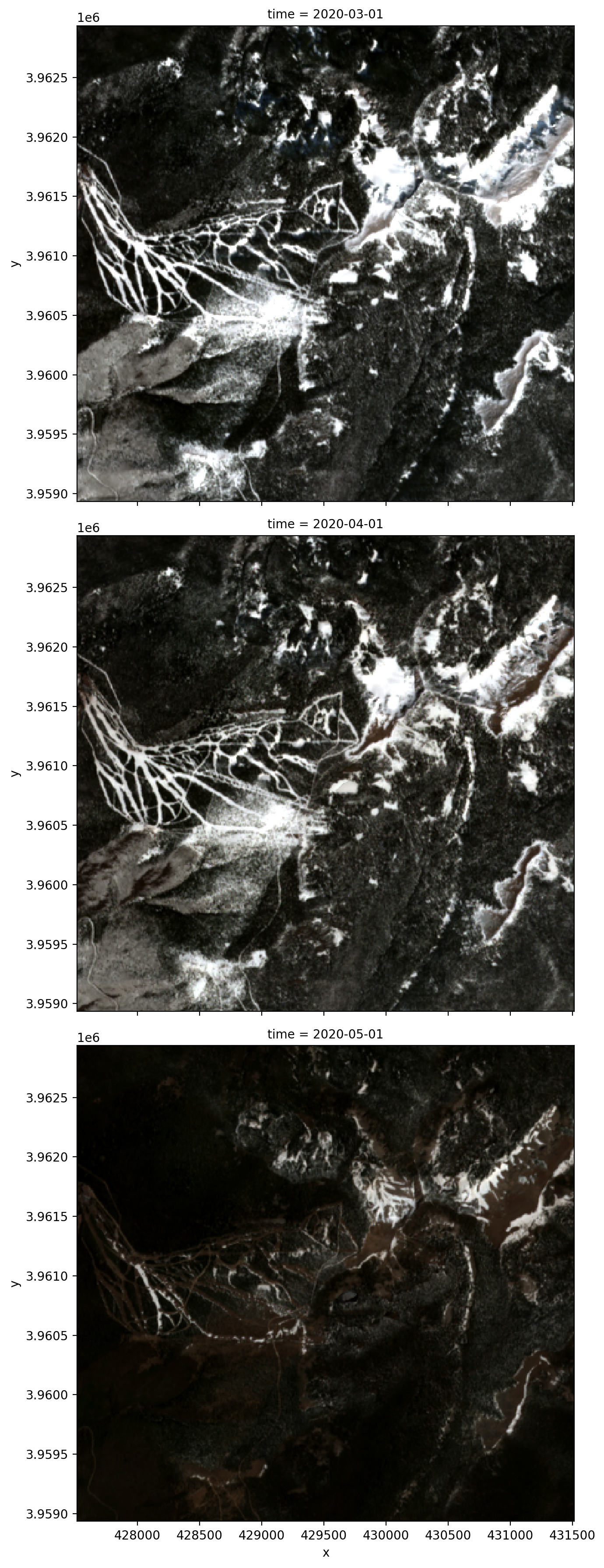
So we don’t pull all ~200 GB of data down to our local machine, let’s slice out a little region around our area of interest.
We convert our lat-lon point to the data’s UTM coordinate reference system, then use that to slice the x and y dimensions, which are indexed by their UTM coordinates.
[9]:
import pyproj
x_utm, y_utm = pyproj.Proj(monthly.crs)(lon, lat)
buffer = 2000  # meters
[10]:
aoi = monthly.loc[..., y_utm+buffer:y_utm-buffer, x_utm-buffer:x_utm+buffer]
aoi
[10]:
<xarray.DataArray 'stackstac-3a21164f19f81366a5242c365d798d31' (time: 3,
                                                                band: 3,
                                                                y: 400, x: 400)>
dask.array<getitem, shape=(3, 3, 400, 400), dtype=float64, chunksize=(1, 1, 387, 316), chunktype=numpy.ndarray>
Coordinates: (12/21)
  * band                                     (band) <U12 'red' 'green' 'blue'
  * x                                        (x) float64 4.275e+05 ... 4.315e+05
  * y                                        (y) float64 3.963e+06 ... 3.959e+06
    s2:product_type                          <U7 'S2MSI2A'
    constellation                            <U10 'sentinel-2'
    mgrs:grid_square                         <U2 'DV'
    ...                                       ...
    gsd                                      (band) object 10 10 10
    common_name                              (band) object 'red' 'green' 'blue'
    center_wavelength                        (band) object 0.665 0.56 0.49
    full_width_half_max                      (band) object 0.038 0.045 0.098
    epsg                                     int64 32613
  * time                                     (time) datetime64[ns] 2020-03-01...
Attributes:
    spec:        RasterSpec(epsg=32613, bounds=(399960.0, 3890220.0, 509760.0...
    crs:         epsg:32613
    transform:   | 10.00, 0.00, 399960.00|\n| 0.00,-10.00, 4000020.00|\n| 0.0...
resolution: 10.0- time: 3
- band: 3
- y: 400
- x: 400
- dask.array<chunksize=(1, 1, 387, 316), meta=np.ndarray>
Array Chunk Bytes 10.99 MiB 0.93 MiB Shape (3, 3, 400, 400) (1, 1, 387, 316) Dask graph 36 chunks in 16 graph layers Data type float64 numpy.ndarray - band(band)<U12'red' 'green' 'blue'
array(['red', 'green', 'blue'], dtype='<U12')
- x(x)float644.275e+05 4.275e+05 ... 4.315e+05
array([427520., 427530., 427540., ..., 431490., 431500., 431510.])
- y(y)float643.963e+06 3.963e+06 ... 3.959e+06
array([3962930., 3962920., 3962910., ..., 3958960., 3958950., 3958940.])
- s2:product_type()<U7'S2MSI2A'
array('S2MSI2A', dtype='<U7') - constellation()<U10'sentinel-2'
array('sentinel-2', dtype='<U10') - mgrs:grid_square()<U2'DV'
array('DV', dtype='<U2') - grid:code()<U10'MGRS-13SDV'
array('MGRS-13SDV', dtype='<U10') - proj:epsg()int6432613
array(32613)
- instruments()<U3'msi'
array('msi', dtype='<U3') - mgrs:latitude_band()<U1'S'
array('S', dtype='<U1') - s2:saturated_defective_pixel_percentage()int640
array(0)
- mgrs:utm_zone()int6413
array(13)
- s2:datatake_type()<U8'INS-NOBS'
array('INS-NOBS', dtype='<U8') - title(band)<U31'Red (band 4) - 10m' ... 'Blue (...
array(['Red (band 4) - 10m', 'Green (band 3) - 10m', 'Blue (band 2) - 10m'], dtype='<U31') - raster:bands(band)objectNone None None
array([None, None, None], dtype=object)
- gsd(band)object10 10 10
array([10, 10, 10], dtype=object)
- common_name(band)object'red' 'green' 'blue'
array(['red', 'green', 'blue'], dtype=object)
- center_wavelength(band)object0.665 0.56 0.49
array([0.665, 0.56, 0.49], dtype=object)
- full_width_half_max(band)object0.038 0.045 0.098
array([0.038, 0.045, 0.098], dtype=object)
- epsg()int6432613
array(32613)
- time(time)datetime64[ns]2020-03-01 2020-04-01 2020-05-01
array(['2020-03-01T00:00:00.000000000', '2020-04-01T00:00:00.000000000',
       '2020-05-01T00:00:00.000000000'], dtype='datetime64[ns]')
- bandPandasIndex
PandasIndex(Index(['red', 'green', 'blue'], dtype='object', name='band'))
- xPandasIndex
PandasIndex(Float64Index([427520.0, 427530.0, 427540.0, 427550.0, 427560.0, 427570.0, 427580.0, 427590.0, 427600.0, 427610.0, ... 431420.0, 431430.0, 431440.0, 431450.0, 431460.0, 431470.0, 431480.0, 431490.0, 431500.0, 431510.0], dtype='float64', name='x', length=400)) - yPandasIndex
PandasIndex(Float64Index([3962930.0, 3962920.0, 3962910.0, 3962900.0, 3962890.0, 3962880.0, 3962870.0, 3962860.0, 3962850.0, 3962840.0, ... 3959030.0, 3959020.0, 3959010.0, 3959000.0, 3958990.0, 3958980.0, 3958970.0, 3958960.0, 3958950.0, 3958940.0], dtype='float64', name='y', length=400)) - timePandasIndex
PandasIndex(DatetimeIndex(['2020-03-01', '2020-04-01', '2020-05-01'], dtype='datetime64[ns]', name='time', freq='MS'))
- spec :
- RasterSpec(epsg=32613, bounds=(399960.0, 3890220.0, 509760.0, 4000020.0), resolutions_xy=(10.0, 10.0))
- crs :
- epsg:32613
- transform :
- | 10.00, 0.00, 399960.00| | 0.00,-10.00, 4000020.00| | 0.00, 0.00, 1.00|
- resolution :
- 10.0
[11]:
import dask.diagnostics
with dask.diagnostics.ProgressBar():
    data = aoi.compute()
[########################################] | 100% Completed | 12.97 s
[13]:
data.plot.imshow(row="time", rgb="band", robust=True, size=6);